
Signal flow graphs (SFG) are the graphical representation of the linear equations. They fulfill important role in circuit analysis, presenting relations between voltages and currents in a clear visible way. Different forms of graphs are already in use. In circuit analysis the most important is Mason signal flow graph representation and only this form will be considered in this work.
1.1. Basic definitions of SFG
Mason SFG is a graphical way of the flow of signals in the circuit. These signals are represented by the variables appearing in linear description of the system [16,20]. They are treated as the nodes in the graph. The nodes are interconnected by the directed arcs, which are often called branches. Each arc is described by its gain (called also transmittance) representing the proper coefficient of the linear equation.
Example 1.1
Let us consider the system of two linear equations
![]() (1.1)
(1.1)
Mason SFG needs presentation of these equations in an explicit form of succeeding variables. In this case it may look like
![]() (1.2)
(1.2)
Now the SFG corresponding to these equations is presented in Fig. 1.1

The internal nodes of the graph are described by the variables xi (i = 1, 2). One node described here by the value 1 represents source node. The only arcs associated with it are going out (the source node cannot have the incoming arcs). The particular nodes are connected with the other nodes by directed arcs, each described by the appropriate gain, representing the coefficient of the linear equation (1.2). Each signal xi of the graph is equal to the sum of incoming signals weighted by the appropriate gain. Any node of the graph can be treated as an output node (variable).
We can recognize the loops, composed of the branches, all of the same direction, forming the closed cycle (without repetition of nodes and branches). The gain of the loop is the product of the gains of the branches forming the closed path. In particular the loop may contain only one branch. In such case it is a self-loop.
Very important advantage of the Mason SFG is the existence of Mason gain formula of the topological nature. It allows calculating any signal xi of the graph treated as the output node. This formula is defined as the transfer function between the signal of the output node and the source node (in the graph of Fig. 1.1 the source node was assumed as 1). This transfer function may be treated as the gain of the system in relation output/input. Let us assume notation [latex]T=\frac{{{X}_{wy}}}{{{X}_{we}}}[/latex], in which Xwy=Xout represents output signal and Xwe=Xin input signal associated with the source node. According to Mason gain formula the transfer function T is described in general as follows [16,20]
 (1.3)
(1.3)
In this equation Δ is the main graph determinant of the graph, which can be presented in the form
![]() (1.4)
(1.4)
The coefficients Gi represent the gains of loops in the graph. The expression for Δ begins with the value of 1. The next term![]() represents the sum of the gains of the loops existing in the graph. The following terms
represents the sum of the gains of the loops existing in the graph. The following terms![]() , etc., represent the gains of non-touching loops combined by two, three, etc. The expansion formula is performed until all non-touching combinations are found. Observe, the following terms of expansion have alternating signs (plus, minus, plus, etc.).
, etc., represent the gains of non-touching loops combined by two, three, etc. The expansion formula is performed until all non-touching combinations are found. Observe, the following terms of expansion have alternating signs (plus, minus, plus, etc.).
The expression [latex]\sum\limits_k T_k \Delta_k[/latex] in the numerator of equations (1.3) represents all forward paths from the source to the output node. Tk means product of the branch gains from the source to the output. Δk is determinant Δ defined for the subgraph which is separated from the kth route. This subgraph is formed by removing the path with all its nodes and arcs. It there are no loops in such subgraph the determinant Δk is identically 1. Mason formula will be illustrated on the example of the graph of Fig. 1.1. Applying this formula we get solution for both variables x1 and x2 in the following forms
[latex]{{T}_{1}}=\frac{{{x}_{1}}}{{{x}_{we}}}=\frac{{{F}_{1}}{{a}_{22}}-{{F}_{2}}{{a}_{12}}}{1-\left[ \left( {{a}_{11}}+1 \right)+\left( {{a}_{22}}+1 \right)+{{a}_{12}}{{a}_{21}} \right]+\left( {{a}_{11}}+1 \right)\left( {{a}_{22}}+1 \right)}[/latex]
[latex]{{T}_{2}}=\frac{{{x}_{2}}}{{{x}_{we}}}=\frac{-{{F}_{1}}{{a}_{21}}+{{F}_{2}}{{a}_{11}}}{1-\left[ \left( {{a}_{11}}+1 \right)+\left( {{a}_{22}}+1 \right)+{{a}_{12}}{{a}_{21}} \right]+\left( {{a}_{11}}+1 \right)\left( {{a}_{22}}+1 \right)}[/latex]
In our example the source node is described by xwe=1, hence the formula delivers direct solution of equations (1.1), because T1=x1, T2=x2. Observe that the procedure of solving this system of equations did not involve any mathematical manipulations with equations of the system.
Example 1.2
As the next example consider the SFG presented in Fig. 1.2, of the gains described by the letters a, b, c, …, l. The variable xwe represents the source node. Let us assume x5 as an output signal.
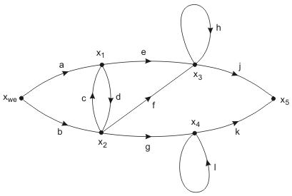
Transfer function T defined as [latex]T = \frac{x_5}{x_{we}}[/latex] is now described in the form
![]()
The main determinant Δ contains three terms associated with the loops (sum of all loop gains, product of the gains of all combinations of two non-touching loops and product of gains of three non-touching loops). The numerator contains 6 terms in the sum, each corresponding to the particular route from the source to the output node x5.
1.2. Application of SFG in analysis of electrical circuits
Mason graph is constructed in general on the basis of the system of linear equations describing the circuit. However, in the case of electrical circuit it is possible to formulate simple rules allowing automatic construction of the graph without describing circuit by the equations. On the other side application of Mason gain formula allows getting solution for any node signal of the circuit. It means that any electrical circuit can be solved by simply inspecting the structure of the analyzed circuit. It leads to the great simplification in analysis of electrical circuits.
To find proper graph representation of the circuit let us consider some typical connection of circuit elements. Let us start from the connection of onl
y passive elements in the kth node as presented in Fig. 1.3a. The symbols V1, V2, …, Vn mean node potentials with respect to the reference node (typically the mass).
|
a)
|
b)
|


Fig. 1.3. Typical connection of passive elements in the kth node (a) and Mason graph corresponding to such connection (b).
From current Kirchhof’s law (nodal description) for this kth node we get
![]() (1.5)
(1.5)
After simple mathematical manipulations we get
![]() (1.6)
(1.6)
where Ysk is the sum of admittances connected to the kth node, ![]() . The equations (1.6) can be associated with the SFG presented in Fig. 1.3b. Observe close similarity of the circuit structure and the graph. Each admittance Yi (i = 1, 2, …, n) of the circuit is represented in the graph by the branch of the gain [latex]\frac{Y_i}{Y_{sk}}[/latex] . Each branch going out from any node Vi (i=1, 2,…,n) is directed toward the node Vk, for which the graph representation is actually constructed. Therefore the graph representation of any node connection in the circuit can be drawn automatically without prior definition of circuit equation for the node.
. The equations (1.6) can be associated with the SFG presented in Fig. 1.3b. Observe close similarity of the circuit structure and the graph. Each admittance Yi (i = 1, 2, …, n) of the circuit is represented in the graph by the branch of the gain [latex]\frac{Y_i}{Y_{sk}}[/latex] . Each branch going out from any node Vi (i=1, 2,…,n) is directed toward the node Vk, for which the graph representation is actually constructed. Therefore the graph representation of any node connection in the circuit can be drawn automatically without prior definition of circuit equation for the node.
This simple passive connection of elements can be easily generalized for more complicated connection of elements involving independent current sources and controlled current sources (nodal description accept only current sources, all other types of sources should be converted to current type using Thevenin-Norton equivalent).
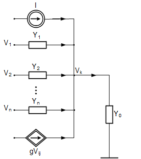
Fig. 1.4a shows such general form of the node containing not only passive elements but also independent current source I and current source controlled by the voltage Vij (voltage between node Vi and Vj). From Kirchhoff’s current law for this node we get
[latex]{{Y}_{1}}({{V}_{1}}-{{V}_{k}})+...+{{Y}_{n}}({{V}_{n}}-{{V}_{k}})+g({{V}_{i}}-{{V}_{j}})+I={{Y}_{0}}{{V}_{k}}[/latex] (1.7)
After simple mathematical manipulation we get the final description of the voltage in node k.
[latex]{{V}_{k}}=\frac{{{Y}_{1}}}{{{Y}_{sk}}}{{V}_{1}}+...+\frac{{{Y}_{n}}}{{{Y}_{sk}}}{{V}_{n}}+\frac{g}{{{Y}_{sk}}}{{V}_{i}}-\frac{g}{{{Y}_{sk}}}{{V}_{j}}+\frac{1}{{{Y}_{sk}}}I[/latex] (1.8)
Once again Ysk is the sum of admittances of passive elements connected to the kth node ![]() . The equations (1.8) is represented in the graph form as shown in fig. 1.4b.
. The equations (1.8) is represented in the graph form as shown in fig. 1.4b.
|
a)
|
b)
|
|
Fig. 1.4. Typical connection of passive elements represented by admittances and current sources in kth node (a) and Mason SFG representing such connection (b). |
|

The interesting simplification in construction procedure is observed in the case of voltage amplifiers, including ideal operational amplifiers (voltage gain tending to infinity). Fig. 1.5 presents the simplified model of voltage amplifier of inverting and non-inverting inputs and the gain A (in the case of ideal operational amplifier the value of A tends to infinity).
| a)
|
b)
|
|
Fig. 1.5. Model of voltage amplifier of inverting and non-inverting inputs (a) and its SFG representation (b) |
|

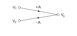
The output voltage Vo of the amplifier is described by
[latex]V_O = AV_1 - AV_2[/latex] (1.9)
The Mason SFG form presented in Fig 1.5b is evident now.
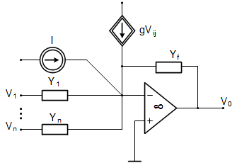
Very often in practical application we deal with special connection of ideal operational amplifiers (A tending to infinity and infinite input impedance), where the noninverting input is grounded. In such case the SFG of the circuit can be greatly simplified.
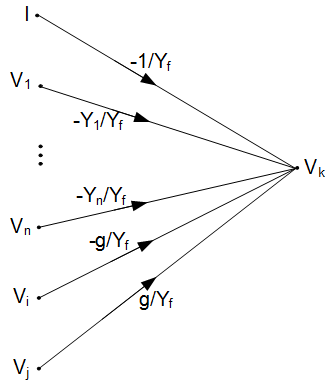
Consider such general case presented in Fig. 1.6a. In such connection of op-amp the potential of non-inverting and inverting node is equal zero. Therefore, from Kirchhoff’s current law written for inverting node we get
[latex]{{Y}_{1}}{{V}_{1}}+...+{{Y}_{n}}{{V}_{n}}+g({{V}_{i}}-{{V}_{j}})+I+{{Y}_{f}}{{V}_{0}}=0[/latex] (1.10)
And finally we are able to obtain expression describing directly the output voltage V0 of the circuit in the following form
[latex]{{V}_{0}}=-\frac{{{Y}_{1}}}{{{Y}_{f}}}{{V}_{1}}+...-\frac{{{Y}_{n}}}{{{Y}_{f}}}{{V}_{n}}-\frac{1}{{{Y}_{f}}}I-\frac{g}{{{Y}_{f}}}{{V}_{i}}+\frac{g}{{{Y}_{f}}}{{V}_{j}}[/latex] (1.11)
The Mason SFG corresponding to such equations is presented in Fig. 1.6b. Once again we can build SFG directly on the basis of inspection of the circuit structure, without writing explicitly Kirchhoff’s equations.
|
a)
|
b)
|
|
Rys. 1.6. Typical general connection of elements containing ideal operational amplifier of infinite gain (a) and Mason SFG corresponding to it (b). |
|
The general procedure of building SFG for the arbitrary circuit structure can be presented in the following way:
-
Recognize all independent nodes in the circuit and denote their nodal voltages.
-
Locate all recognized nodes of the future graph in the configuration similar to their positions in the circuit. Recognize the source node, from which only out-going branches are possible (there is no need to build its graph representation).
-
Step by step build the graph representation for the succeeding nodes using their associated SFG represented in figures 1.3 – 1.6.
-
In general case for the limited gain A of the amplifier (different from infinity) we must recognize two cases:
-
The node under construction is placed on the output of op-amp. In such case use its general model of Fig. 1.5.
-
Else, if the node is not on the output of op-amp – use its models presented in Fig. 1.3 or 1.4.
-
-
In the case of infinite gain of op-amp you may apply the previous model of op-amp and finally calculate the limit of final expression of transfer function at A tending to infinity, or use the simplified model of op-amp shown in Fig. 1.6.
-
Remember, in constructing SFG representation of particular node the appropriate branches should directed to this node. After traveling through all nodes of the circuit the final form of the graph is created.
1.3. Examples of SFG application in analysis of circuits with operational amplifiers
1.3.1 Filter structure with multiloop feedback
The procedure described above will be illustrated on the example of multiloop feedback circuit very often used in filter design (Fig. 1.7a). Assume gain of ideal op-amp equal infinity. Because the noninverting node is grounded the node potential V2 is zero and will not appear in SFG. Therefore, we use the simplified model of op-amp presented in Fig. 1.6b.
|
a)
|
|
b)
|
| Fig.. 1.7. Multiloop filter structure (a) and Mason SFG corresponding to such circuit (b). |
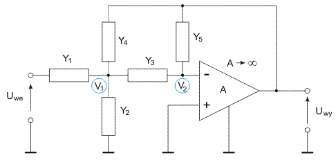
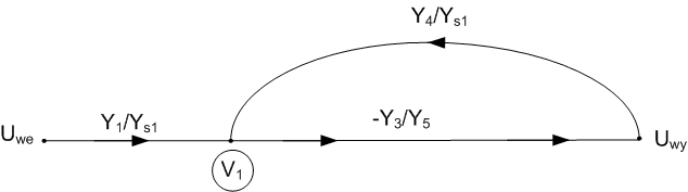
The circuit contains three nodes (V1, V2 and Uwy), from which V2=0 and will not appear in the graph. The graph representation of the circuit is created for each node (V1, and Uwy) in an independent way.
Node V1 is a typical connection of passive elements and therefore, its graph of Fig. 1.3 is applied. Node V2=0 is excluded from the graph. Graph representation of Uwy follows from the model illustrated on Fig. 1.6. Fig. 1.7b shows the final form of the graph. Applying Mason gain formula we get the following transfer function
[latex]T=\frac{{{U}_{wy}}}{{{U}_{we}}}=\frac{-\frac{{{Y}_{1}}{{Y}_{3}}}{{{Y}_{s1}}{{Y}_{5}}}}{1+\frac{{{Y}_{3}}{{Y}_{4}}}{{{Y}_{s1}}{{Y}_{5}}}}=\frac{-{{Y}_{1}}{{Y}_{3}}}{{{Y}_{5}}{{Y}_{s1}}+{{Y}_{3}}{{Y}_{4}}}[/latex] (1.12)
where ![]() . After substituting the expression for Ys1 we get the final form of solution
. After substituting the expression for Ys1 we get the final form of solution
[latex]T=\frac{-{{Y}_{1}}{{Y}_{3}}}{{{Y}_{5}}\left( {{Y}_{1}}+{{Y}_{2}}+{{Y}_{3}}+{{Y}_{4}} \right)+{{Y}_{3}}{{Y}_{4}}}[/latex] (1.13)
Applying proper description of elements in s-domain (for resistor Y=1/R, for capacitor Y=sC, for inductor Y=1/sL) we get the typical transfer function of complex frequency s, T=T(s)=H(s) being the starting point in filter design.
1.3.2 Circuits with voltage amplifiers of finite gain
As an example consider the circuit structure containing five voltage amplifires of the finite gains: K1, K2, K3, K4 and K5 as shown in Fig. 1.8a. Transfer function of the circuit is defined as T=Uwy/Uwe [16].
|
a)
|
|
b)
|
| Fig. 1.8. The circuit structure with voltage amplifiers of finite gain (a) and Mason SFG corresponding to this circuit (b). |
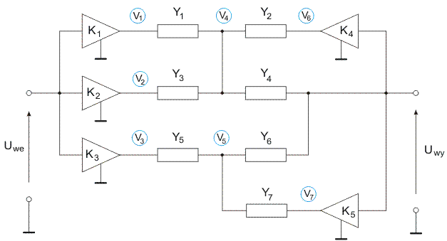
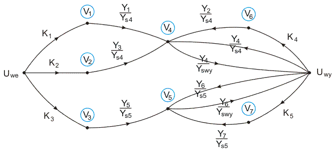
The SFG, constructed according to the presented procedure, is shown in Fig. 1.8b. After application of Mason gain formula we get transfer function T in the form.
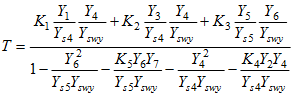 (1.14)
where ![]() ,
, ![]() ,
, ![]() . After simplification we get the final form
. After simplification we get the final form
latex T=\frac{\left( {{K}_{1}}{{Y}_{1}}{{Y}_{4}}+{{K}_{2}}{{Y}_{3}}{{Y}_{4}} \right){{Y}_{s5}}+{{K}_{3}}{{Y}_{5}}{{Y}_{6}}{{Y}_{s4}}}{{{Y}_{s4}}{{Y}_{s5}}{{Y}_{swy}}-Y_{6}^{2}{{Y}_{s4}}-{{K}_{5}}{{Y}_{6}}{{Y}_{7}}{{Y}_{s4}}-Y_{4}^{2}{{Y}_{s5}}-{{K}_{4}}{{Y}_{2}}{{Y}_{4}}{{Y}_{s5}}}$ (1.15)
After declaring particular forms of elements (for example resistor Y=1/R, capacitor Y=sC) we obtain the typical transfer function of complex frequency s, T=T(s).
1.3.3. Biquadratic structure containing three operational amplifiers
Let us consider the so called biquadratic structure built on the basis of three operational amplifiers and RC elements, as shown in Fig. 1.9a. The voltage transfer function of the circuit is defined as [latex]T(S) = \frac{U_{wy}}{U_{we}}[/latex] . We will build the SFG using model of op-amp of finite gain A, as presented in Fig. 1.5.
| a)
|
|
b)
|
| Fig. 1.9. The structure of biquadratic filter (a) and its SF (b) |
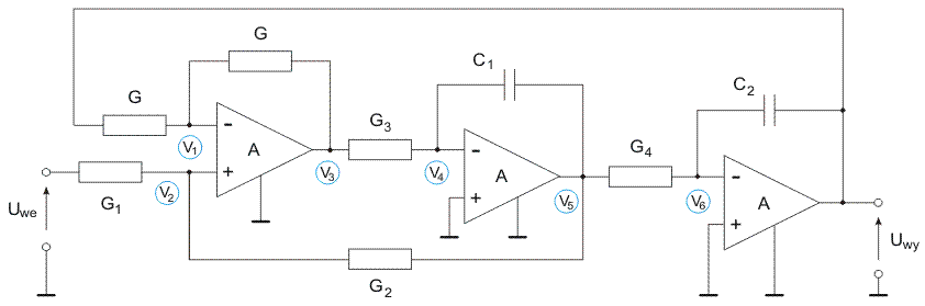

The Mason SFG built at the assumption of finite gain of operational amplifier is presented in Fig. 1.9b. It contains 5 loops, within which we can recognize some combination of two non-touching loops and even three non-touching loops. Applying Mason gain formula we get
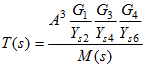 (1.16)
of the denominator M(s) given in the form
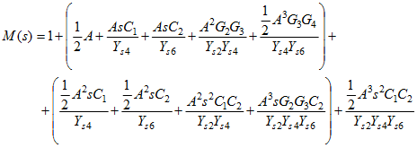 (1.17)
This general solution can be significantly simplified if we assume the gain A tending to infinity, [latex]A \to \infty[/latex] . In such case we get
![]() (1.18)
(1.18)
1.3.4. KHN filter structure
The next example will consider the biquadratic structure defined by Kervin-Huelsman-Newcomb (KHN) shown in fig. 1.10a containing operational amplifiers of infinite gain [16]. This is the structure similar to the already analyzed in the previous section. This time we apply the simplified model of infinite gain operational amplifier of grounded non-inverting inputs.
| a)
|
| b)
|
| Fig. 1.10. KHN filter structure (a) and Mason SFG corresponding to this structure (b).
|
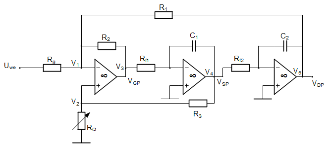
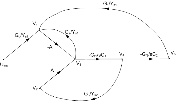
Fig. 1.10b presents SFG of the circuit. Applying Mason gain formula we obtain solution in the form of appropriate transfer function. Assuming different output nodes three different transfer functions T(s) can be obtained. They are defined in the following forms
[latex]{{T}_{LP}}(s)=\frac{{{V}_{5}}}{{{U}_{we}}}=\frac{-\frac{{{R}_{2}}}{{{C}_{1}}{{C}_{2}}{{R}_{f1}}{{R}_{f2}}{{R}_{g}}}}{M(s)}[/latex] (1.19)
[latex]{{T}_{BP}}(s)=\frac{{{V}_{4}}}{{{U}_{we}}}=\frac{s\frac{{{R}_{2}}}{{{C}_{1}}{{R}_{f1}}{{R}_{g}}}}{M(s)}[/latex] (1.20)
[latex]{{T}_{HP}}(s)=\frac{{{V}_{3}}}{{{U}_{we}}}=\frac{-{{s}^{2}}\frac{{{R}_{2}}}{{{R}_{g}}}}{M(s)}[/latex] (1.21)
All transfer functions have the same denominator M(s). It is a polynomial of the second order defined as following (conductance G are inverses of the proper resistances)
[latex]M(s)={{s}^{2}}+s\frac{{{R}_{2}}({{G}_{1}}+{{G}_{2}}+{{G}_{g}})}{{{C}_{1}}{{R}_{3}}{{R}_{f1}}({{G}_{3}}+{{G}_{Q}})}+\frac{{{R}_{2}}}{{{C}_{1}}{{C}_{2}}{{R}_{1}}{{R}_{f1}}{{R}_{f2}}}[/latex] (1.22)
From these expressions it is evident that transfer function TLP(s) represents the lowpass filter, TBP(s) – bandpass filter and THP(s) – high-pass filter.
1.3.5. FDNR circuit
Mason graphs built for the circuits, according to the presented procedure, are based on nodal description of the circuit and operate only by voltages. In the case when the output variable is a current the additional node of the graph representing the current is needed. The representation of such node is created using the Kirchhoff’s law, in which the current is expressed through the nodal voltages.
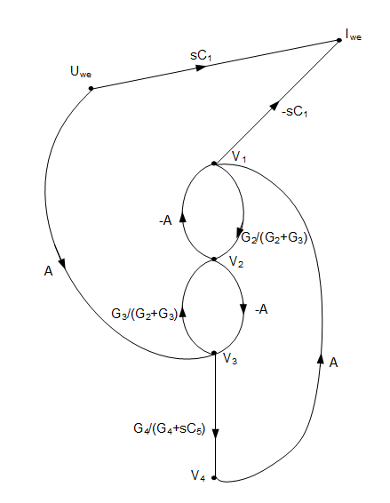
The example of such case will be presented for the circuit called Frequency Dependent Negative Resistor (FDNR). FDNR represents the input admittance Ywe=Y(s)=Ds2 , of the positive coefficient D. The structure of FDNR is depicted on Fig. 1.11a. It contains two ideal operational amplifiers, three resistors and two capacitors [4,16].
| a)
|
b)
 |
|
Fig. 1.11. Structure of FDNR (a) and Mason SFG for computing the input admittance (b). |
|
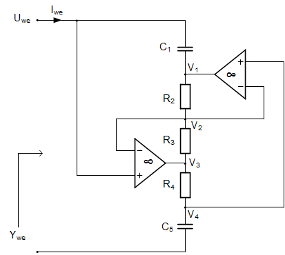
In the case of admittance the output node represents the input current and the source node is the input voltage, since Y(s)=Iwe/Uwe. Assuming ideal operational amplifiers of infinite input impedance the input current Iwe can be expressed in the form
Iwe=sC(Uwe-V1) (1.23)
The SFG for such circuit is built in the same way as for the previous circuits. The only difference is in output node, which is built on the basis of eq. (1.23). Full structure of SFG is shown in Fig. 1.11b, in which the input current is denoted by Iwe and input voltage by Uwe. Application of Mason gain formula leads to the solution of the following form, dependent on the arbitrary value of operational amplifier gain A.
[latex]Y(s)=\frac{s{{C}_{1}}\Delta +{{A}^{2}}s{{C}_{1}}\frac{{{G}_{3}}}{{{G}_{2}}+{{G}_{3}}}-{{A}^{2}}s{{C}_{1}}\frac{{{G}_{4}}}{{{G}_{4}}+s{{C}_{5}}}}{\Delta }[/latex] (1.24)
where the main determinant Δ is given by
[latex]\Delta =1+A\frac{{{G}_{3}}}{{{G}_{2}}+{{G}_{3}}}+A\frac{{{G}_{2}}}{{{G}_{2}}+{{G}_{3}}}+{{A}^{2}}\frac{{{G}_{2}}}{{{G}_{2}}+{{G}_{3}}}\frac{{{G}_{4}}}{{{G}_{4}}+s{{C}_{5}}}[/latex] (1.25)
Assuming [latex]A \to \infty[/latex] the expression for Y(s) is simplified to
[latex]Y(s)={{s}^{2}}\frac{{{C}_{1}}{{C}_{5}}{{G}_{3}}}{{{G}_{2}}{{G}_{4}}}={{s}^{2}}\frac{{{C}_{1}}{{C}_{5}}{{R}_{2}}{{R}_{4}}}{{{R}_{3}}}[/latex] (1.26)
Comparing this expression with the definition of FDNR Y(s)=Ds2 we find the value of coefficient D as follows
[latex]D=\frac{{{C}_{1}}{{C}_{5}}{{R}_{2}}{{R}_{4}}}{{{R}_{3}}}[/latex] (1.27)
This value depends only on the parameters of the passive elements (the resistors and capacitors). Observe, that in steady state operation at sinusoidal excitation of the angular frequency ω, the FDNR represents the negative conductance controlled by the frequency, since in such case Y(s=jω)=G=-ω2C1C5R2R4/R3.
1.4 Exercises
-
Draw signal flow graph for the system of linear equations
[latex]{{x}_{1}}=2{{x}_{1}}+3{{x}_{2}}+4{{x}_{3}}[/latex]
[latex]{{x}_{2}}=-4{{x}_{1}}+5{{x}_{3}}+10[/latex]
[latex]{{x}_{3}}={{x}_{1}}-2{{x}_{2}}+6{{x}_{3}}+5[/latex]
Solution:
Graph corresponding to this system of linear equations is presented in Fig. 1.12
 |
| Fig. 1.12 Signal flow graph representing the system of linear equations |
- Draw signal flow graph for the given circuit and calculate V3
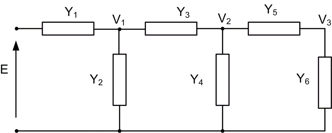 |
| Fig. 1.13a The circuit structure |
Solution:
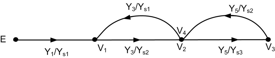
SFG representing the nodal circuit equations for circuit of Fig. 1.2a is shown in Fig. 1.2b.
The admittances included in the graph are equal:
Ys1=Y1+Y2+Y3
Ys2=Y3+Y4+Y5
Ys3=Y5+Y6
From Mason formula we get the expression for voltage V3 as follows
[latex]{{V}_{3}}=E\frac{\sum\limits_{k}^{{}}{{{T}_{k}}{{\Delta }_{k}}}}{\Delta }=E\frac{{{Y}_{1}}{{Y}_{3}}{{Y}_{5}}}{1-Y_{3}^{2}/{{Y}_{s1}}{{Y}_{s2}}-Y_{5}^{2}/{{Y}_{s2}}{{Y}_{s3}}}=E\frac{{{Y}_{1}}{{Y}_{3}}{{Y}_{5}}}{{{Y}_{s1}}{{Y}_{s2}}{{Y}_{s3}}-Y_{3}^{2}{{Y}_{s3}}-Y_{5}^{2}{{Y}_{s1}}}[/latex]
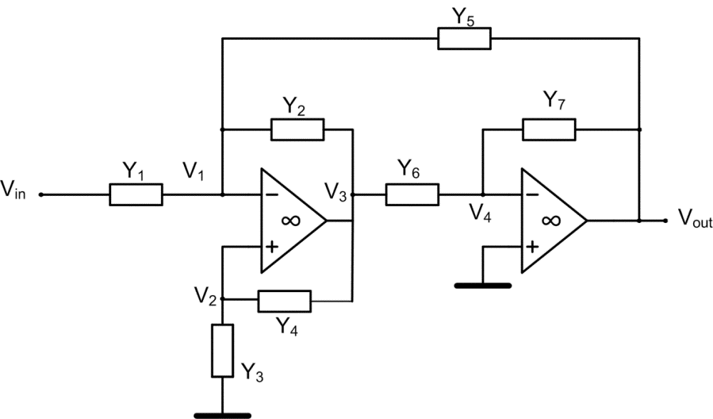
Apply signal flow graph to calculate transfer function T=Vout/Vin at the gain of operational amplifier A→∞
 |
Solution:
SFG corresponding to the circuit structure of Fig. 1.3a is presented in Fig. 1.3b, where Ys1=Y1+Y2+Y5.
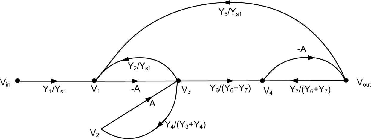
From Mason formula we obtain
[latex]T=\frac{\sum\limits_{k}^{{}}{{{T}_{k}}{{\Delta }_{k}}}}{\Delta }=\frac{{{A}^{2}}\frac{{{Y}_{1}}}{{{Y}_{s1}}}\frac{{{Y}_{6}}}{{{Y}_{6}}+{{Y}_{7}}}}{1-\left( -\frac{A{{Y}_{2}}}{{{Y}_{s1}}}+\frac{A{{Y}_{4}}}{{{Y}_{3}}+{{Y}_{4}}}-\frac{A{{Y}_{7}}}{{{Y}_{6}}+{{Y}_{7}}}+\frac{{{A}^{2}}{{Y}_{5}}{{Y}_{6}}}{{{Y}_{s1}}\left( {{Y}_{6}}+{{Y}_{7}} \right)} \right)+\left( \frac{{{A}^{2}}{{Y}_{2}}{{Y}_{7}}}{{{Y}_{s1}}\left( {{Y}_{6}}+{{Y}_{7}} \right)}-\frac{{{A}^{2}}{{Y}_{4}}{{Y}_{7}}}{\left( {{Y}_{3}}+{{Y}_{4}} \right)\left( {{Y}_{6}}+{{Y}_{7}} \right)} \right)}[/latex]
Assuming A→∞ we get
[latex]{{T}_{\infty }}=\frac{{{Y}_{1}}{{Y}_{6}}\left( {{Y}_{3}}+{{Y}_{4}} \right)}{{{Y}_{2}}{{Y}_{7}}\left( {{Y}_{3}}+{{Y}_{4}} \right)-{{Y}_{5}}{{Y}_{6}}\left( {{Y}_{3}}+{{Y}_{4}} \right)-{{Y}_{4}}{{Y}_{7}}\left( {{Y}_{1}}+{{Y}_{2}}+{{Y}_{5}} \right)}[/latex]
1.5 Basic definitions
Branch – the directed arch joining two nodes in the graph.
Branch gain – the gain parameter associated with the branch. The output node signal of the branch is its input node signal multiplied by this gain.
FDNR – frequency dependent negative resistor, i.e., the electronic circuit implementing negative resistance controlled by the frequency.
Forward path – a path from an input node to an output node in which no node is touched more than once.
Gain of graph – the ratio of output signal to the input (source) signal calculated by Mason gain formula. It is also called transfer function.
Graph determinant – the mathematical expression used in Mason gain formula. It is formed on the basis of the loop gains existing in the graph.
Graph model of circuit – graph representation of the circuit equations, built usually by inspection of the circuit without declaring the Kirchhoff’s description in an explicit way.
Loop – a closed path of directed branches. It originates and ends on the same node, and no node is touched more than once).
Loop gain – the product of the gains of all the branches in the loop.
Mason’s gain formula – the method for finding the transfer function from the source to the output node of a linear signal-flow graph.
Non-touching loops – the loops having no common nodes.
Path – the continuous set of branches traversed in the direction indicated by the branch arrows.
Path gain – the product of the gains of all the branches in the path.
Self-loop – the branch, which begins and ends at the same node without entering other nodes.
Signal flow graph – the graphical representation of the linear system of equations in which variables are represented by nodes and coefficients by the gains of archs joing two nodes.