2 Low frequency current and voltage disturbances

Definition of electromagnetic disturbance, named shortly disturbance in these lecture notes is inserted in sub chapter [EU regulation]. Another relevant definition is interference which is unwanted impact of the electromagnetic disturbance on other arrangements energized electrically. Disturbance is cause and interference is effect.

Disturbance can be for instance sparking on the commutator of the brush motor in the hair dryer or drilling machine, that can interfere radio receiver or garage door opener.

There are two kind of origins (of sources) of the electromagnetic disturbance: Man and Nature. Man-made disturbance can be either side effect of operation of arrangement or can be intentional.

It is commonly known that AC/AC inverters widespread in power electronic are source of nasty radio frequency disturbances which are unwanted side effect of their operation.

Purpose of intentional sources of disturbances can be peaceful or military.

Two examples of intentional, peaceful sources of disturbances:

1. electro erosion machine tool is equipped with high voltage source which generates intentionally electric arc to form parts by removing metal chips from a workpiece, but electromagnetic field accompanying the arc can interfere other arrangements in the surroundings,
2. mobile telephone communicates with radio signal which is intentional and useful for someone who wants to talk on the mobile phone but this radio signal can be disastrous for an aircraft especially by takeoff and landing.

Unfortunately Man uses also electromagnetic energy intentionally as a weapon. High power microwaves or Nuclear Electromagnetic Pulse are example of that. They are called “humanitarian” weapons.

Disturbances can be classified in respect to different features:

• frequency – low frequency (e.g. voltage flicker in public electricity network), radio frequency (e.g. glow discharge in a gas-discharge lamp),
• frequency band – narrowband (e.g. radiation of microprocessor by its operating frequency or harmonics of it), wideband (e.g. radio frequency RF propagation from the switched mode power supply SMPS¹),
• inherent energy – low energy (e.g. electrostatic discharge), high energy (e.g. lightning electromagnetic pulse LEMP),
• dwell time – transient event (e.g. commutation notches) or continuous event (e.g. power frequency magnetic field in the vicinity of house electrical installation.

Current harmonics

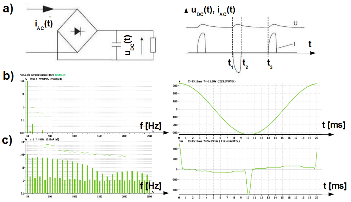
Rectifier is inherent module in the front end of majority of electronic devices. It is essential source of current harmonics. An example is discussed below.

In Fig.2.1 a) two-pulse rectifier is shown. From the instant [latex]t_1[/latex] on, instantaneous rectified voltage is bigger than condenser voltage. Condenser is charged with the current drawn from the AC source. Charging stops in the instant [latex]t_2[/latex] when instantaneous rectified voltage becomes smaller than condenser voltage. Condenser begins to discharge with the time constant [latex]RC[/latex]. Current is not drawn anymore from the AC source. Discharge lasts till the instant [latex]t_3[/latex] which is the end of charging-discharging period. The AC current is drawn in the short time interval [latex]t_2 - t_1[/latex] by the peak value of the AC voltage. The bigger time constant [latex]RC[/latex] the shorter is the current impulse drawn from the AC source.

In Fig.2.1 c) on the right, current for such rectifier measured in the time domain is shown. Such current in the frequency domain is characterized with very big content of odd harmonics. In this case the [latex]3^{rd}[/latex], [latex]5^{th}[/latex], [latex]7^{th}[/latex] and [latex]9^{th}[/latex] are bigger than [latex]80\%[/latex] of the main harmonic, see the left of Fig.2.1. The frequency range of interest is up to 40-th harmonic e.i. up to 2 [latex]kHz[/latex] by 50 [latex]Hz[/latex] supply network.

For measurements of current harmonics the AC source with practically zero internal impedance must be used. Voltage at the AC input of rectifier shown in the frequency and time domain in Fig.2.1 b) is practically free of harmonics. It means that origin of measured current harmonics is solely rectifier but not interaction of the rectifier and AC source impedance.

Flicker

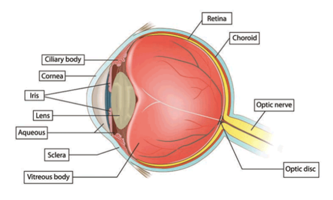
If the light flux captured by eye changes, retina sends signal with optic nerve to the brain, see Fig.2.2. Feed back of the brain is to activate muscles of iris in order to adjust pupil size to the flux. Single flux change is not remarkable by the Man. However repetitive changes of the light flux, called light flicker, shadow flicker or just flicker can cause physiological discomfort, physical and psycho tiredness by healthy people up to inducing epileptic seizures by people who suffer from photosensitive epilepsy. Scale of impact depends on repetition rate and depth of the flux changes.

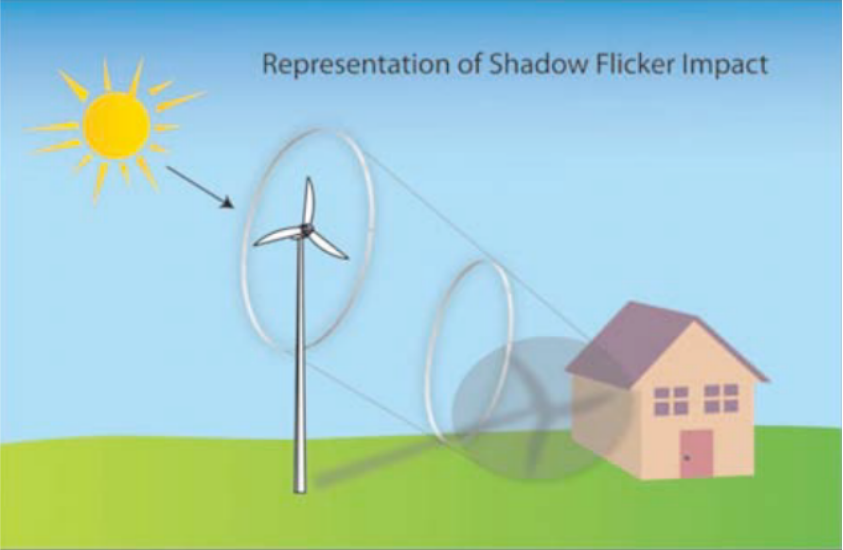
There are different origins of flicker. One of them is the wind turbine. Shadow flicker occurs when the sun is low in the sky and a wind turbine creates a shadow on a building Fig.2.3. As the turbine blades pass in front of the sun, a shadow moves across the landscape, appearing to flick on and off as the turbine rotates. The location of the turbine shadow varies by time of day and season and usually only falls on a single building for a few minutes of a day. Shadows that fall on a home may be disruptive. Shadow flicker has been a concern in Northern Europe where the high latitude and low sun angle exacerbate the effect [@Shadow; @flicker].

The intermittent shadows can also experience a car driver driving along a tree lined street or in a road tunnel lighted with lamps mounted with spacing.

The concern of this lecture notes is flicker caused by light flux changes due to power delivered to the electric lighting. This power is proportional to the Root Mean Square RMS value of supply voltage therefore flicker is equalized with changes of the RMS voltage.

In rural areas by long distances to the transformer, low voltage public electricity networks is weak. It has relatively big impedance. If in such area one consumer switches ON/OFF for instance electrical welding machine, his neighbors sens it as repetitive changes of the RMS of supply voltage, actually flicker.

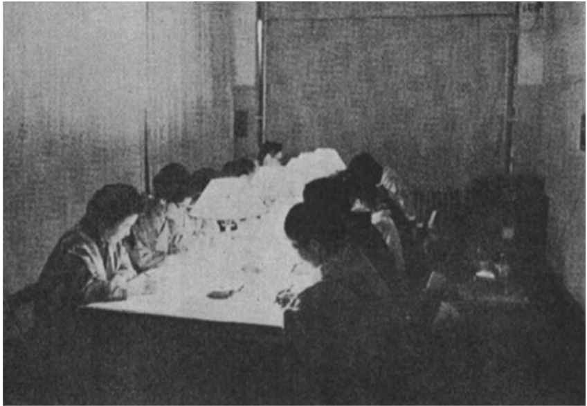
In [latex]80^{th}[/latex] of [latex]20^{th}[/latex] century many experiments were done on different groups of people exposed to the flicker of the electric light. 60 [latex]W[/latex] incandescent bulbs were used as a flickering light source. Picture of probants by such experiment is shown in Fig Fig.1.4. It was agreed for 10 [latex]min[/latex] observation time.

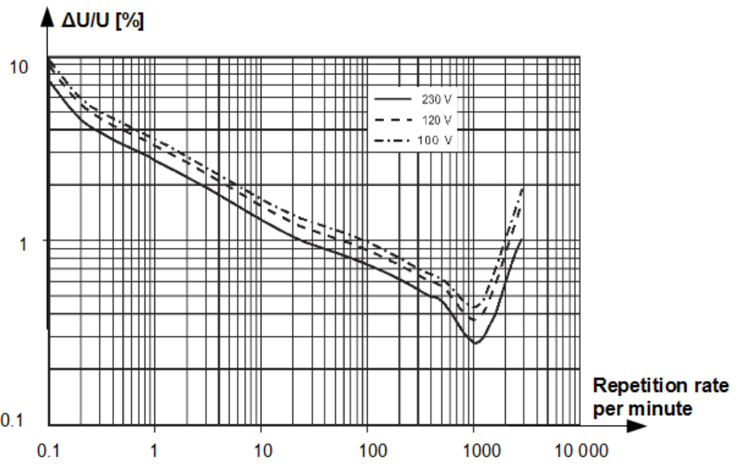
Result of that experiments are curves of the short time flicker factors [latex]P_{st}[/latex] shown in Fig.1.5. There are three curves for 100[latex]V[/latex], 120[latex]V[/latex] and 230[latex]V[/latex] rated voltage. Value [latex]P_{st} = 1[/latex] is assigned to them. The region below is tolerable, above is considered as disruptive. Remarkable is that this phenomenon has extremely low frequency. Plots ends by 50 [latex]Hz[/latex]. Moreover very small relative changes of the RMS voltage are critical. Most sensitive region is by 1000 changes per minute i.e. by 16.6 [latex]Hz[/latex] by which changes below 0.3[latex]\%[/latex] are already critical (by 230 [latex]V[/latex] rated voltage).

In addition to the short time flicker factor [latex]P_{st}[/latex], the long time flicker factor [latex]P_{lt}[/latex] is defined. It is indispensable because there are processes which last for a longer time e.g. washing machine programs which can last up to two hours. During that time current consumption goes up and down due to sequence of different operations: water drawing, heating, tumbling, drying, water pumping down etc.. [latex]P_{lt}[/latex] is defined as follows

[latex]P_{lt} = \left[ \frac{\sum_{i=1}^N P_{st_i}^{3}} {N} \right]^{\frac{1}{3}} \label{Plt}\tag{2.1}[/latex]

where [latex]P_{st_i}[/latex] is the short time flicker factor observed in the i-th 10 [latex]min[/latex] time segment and [latex]N[/latex] is the number of observed time segments.

Characteristic of main’s voltage

Origin of phenomena described before: current harmonics and flicker are arrangements supplied by the public electricity network. These disturbances are emitted from the arrangement to the environment, to the public electricity network. Interaction is mutual. Disturbances in the public electricity network can influence the arrangements supplied from it. The standard [@EN-50160] is devoted to characterizing the quality of the main’s voltage. The main features of this quality are: flicker, harmonics, unbalance, commutation notches, dips, interruptions and variations. Flicker, unlike remaining features do not need any additional informations.

The quality of voltage is characterized in so called supply terminal which is point in a public supply network designated as such and contractually fixed, at which electrical energy is exchanged between contractual partners [@EN-50160] i.e. at the input of energy meter by the consumer.

Harmonics

Voltage total harmonic distortion [latex]THD_U[/latex] defined as quotient of root of sum of squares RSS of all harmonics to fundamental harmonic [latex]U_1[/latex] is used as distortion measure

[latex]THD_U = \frac{\sqrt{\sum_{n=1}^{40} U_n^{2}}} {U_1} \label{THD}\tag{2.5}[/latex]

Sometimes THD is split to odd harmonic distortion OHD

[latex]OHD_U = \frac{\sqrt{\sum_{n=1}^{19} U_{2n+1}^{2}}} {U_1} \label{THDa}\tag{2.5}[/latex]

and even harmonic distortion EHD

[latex]EHD_U = \frac{\sqrt{\sum_{n=1}^{20} U_{2n}^{2}}} {U_1} \label{THDb}\tag{2.5}[/latex]

Understandably THD is geometric sum of OHD and EHD

[latex]THD_U = \sqrt{OHD_U^2 + EHD_U^2} \label{THDc}\tag{2.5}[/latex]

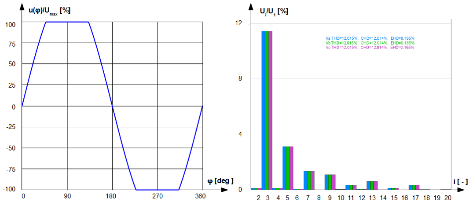
In Fig.1.6 decapitated sinus voltage with [latex]THD=12\%[/latex] is shown. Remarkable is dominant contribution of OHD. EHD is practically negligible. Moreover RMS value of this voltage is only slightly increased by distortion [latex]U_{_{RMS}} \approx 1.007 \cdot U_{1_{RMS}}[/latex].

Unbalance

Any three phase unbalanced voltage system can be decomposed into: plus, minus and zero component as shown in Fig.1.7.

Phasors of positive components rotate counterclockwise in sequence: [latex]U_{A_P}[/latex], [latex]U_{B_P}[/latex], [latex]U_{C_P}[/latex] on the complex plane

[latex]U_{A_P} = |U_P|e^{j\omega t} \label{UAP} \tag{2.6}[/latex]

[latex]U_{B_P} = |U_P|e^{ - j120^\circ} e^{j\omega t} \label{UBP} \tag{2.7}[/latex]

[latex]U_{C_P} = |U_P|e^{ j120^\circ} e^{j\omega t} \label{UCP} \tag{2.8}[/latex]

Phasors of negative components rotate counterclockwise in sequence: [latex]U_{A_P}[/latex], [latex]U_{C_P}[/latex], [latex]U_{B_P}[/latex] on the complex plane

[latex]U_{A_N} = |U_N|e^{j\omega t} \label{UAN} \tag{2.9}[/latex]

[latex]U_{B_N} = |U_N|e^{ j120^\circ} e^{j\omega t} \label{UBN} \tag{2.10}[/latex]

[latex]U_{C_N} = |U_N|e^{ -j120^\circ} e^{j\omega t} \label{UCN} \tag{2.11}[/latex]

Phasors of zero components rotate on the complex plane without phase shift

[latex]U_{A_0} = U_{B_0} = U_{C_0} = |U_0|e^{j\omega t} \label{U0}\tag{2.12}[/latex]

Voltage unsymmetry factor [latex]VUF_N[/latex] of the negative component defined as

[latex]VUF_N = \frac{|U_N|}{|U_P|} \label{UVFN}\tag{2.13}[/latex]

and voltage unsymmetry factor of the zero component [latex]VUF_0[/latex] defined as

[latex]VUF_0 = \frac{|U_0|}{|U_P|} \label{UVF0}\tag{2.14}[/latex]

are unsymmetry measures.

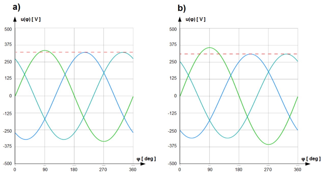
In Fig.1.8 a) and b) three phase unsymmetrical voltage system with [latex]VUF_N = 3\%[/latex] and [latex]VUF_N = 10\%[/latex] respectively, free of zero component ([latex]VUF_0 = 0\%[/latex]) are shown.

Dips and interruptions

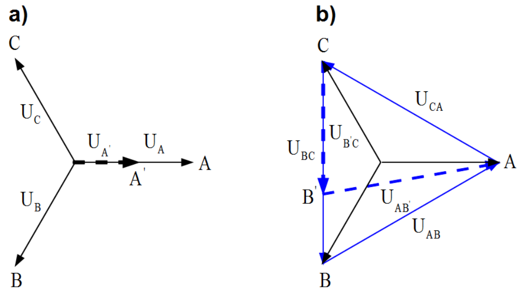
Dips of interest depends on whether loads in the arrangement are supplied with line to neutral or line to line voltage. In Fig.1.9 a) line to neutral voltage [latex]U_A[/latex] is reduced. The residual voltage [latex]U_{A^{'}}[/latex] is shown as dashed arrow.

In Fig.1.9 b) line to line voltage [latex]U_{BC}[/latex] is reduced. The residual voltage [latex]U_{B^{'}C}[/latex] is shown as dashed arrow. This dip has impact also on [latex]U_{AB}[/latex] voltage which becomes [latex]U_{{AB}^{'}}[/latex] (dashed arrow).

Dwell time of dips is expressed in fold of a period. Additionally dip with [latex]0V[/latex] residual voltage and half of a period dwell time is of interest due to risk of saturation of chokes in the front end of the appliances.

Two features distinguish voltage interruption from dip: it is longer phenomenon, measured in seconds and the rest voltage is [latex]0V[/latex] in all lines simultaneously.

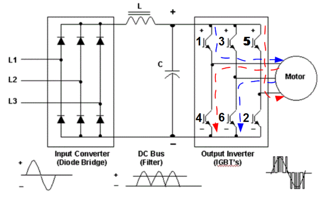
Commutation notches

Output inverter in the frequency drive is composed of three columns with pair of valves (IGBTs in Fig.1.10) 1-4, 3-6, 5-2 or recently valves built in Silicon Carbon Technology SiC. They are operated in such sequence that never vales from the same column should be closed. For example if in one instant valves 1-6 are closed (blue dashed line), in the next 5-4. It will surely be the case if commutation (state transition of the valve) would have unchangeable rise and fall time. Unfortunately duration of commutation can vary randomly. As a cause valve for instance 1 will be not yet totally opened while valve 4 will be already partly closed. On the AC side of the drive such situation looks like a short circuit for a short instance of the time, fraction of miliseconds. For other consumers it can be sensed as short time dip in supply voltage as shown in Fig.1.10. This phenomenon is called commutation notch.

Solar storm {#Solar storm}

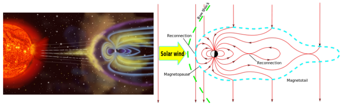
There is continuous eruption of plasma from the Sun’s surface. A stream of it released from the upper atmosphere of the Sun builds so called solar wind. Plasma embedded within the solar wind is the interplanetary magnetic field called also magnetic cloud. If the material carried by the solar wind reached a planet’s surface, its radiation would do severe damage to any life that might exist. Earth’s magnetic field serves as a shield, redirecting the material around the planet so that it streams beyond it. If the stream is constant in time, interplanetary magnetic cloud and Eart’s magnetosphere are in equilibrium.

However the Sun’s activity shifts over the course of its 11-year cycle with radiation levels, and ejected material changing over time. These alterations affect the properties of the solar wind, including its magnetic field. This phenomenon is called solar storm.

Time dependent magnetic field of the interplanetary magnetic cloud stretches out the Eart’s magnetosphere so that it is smoothed inward on the sun-side and stretched out on the night side, see Fig. 1.12. The duration of the main phase of the storm is typically 2 – 8 hours. The recovery phase may last as short as 8 hours or as long as 7 days.

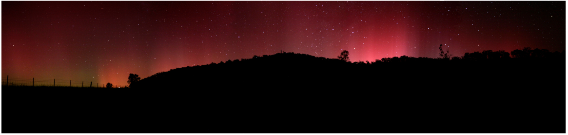
Aurora phenomenon observable usually in the polar circles can be observed by solar storm in much smaller latitudes eg. in Australia, see Fig. 1.13. But there are more severe influences of the solar storm on our civilization.

According to Faraday’s law [@Hammond] changes of magnetic flux generates electromotive force EMF in any metal structure comprising the flux

[latex]EMF = - \frac{d \phi (t)}{dt} = - \mu_0 \frac{ d\left( \int_{S} \overrightarrow{H} (t) \cdot d\overrightarrow{S}\right)}{dt} \label{Faraday}\tag{2.15}[/latex]

where S is area which flux is crossing.

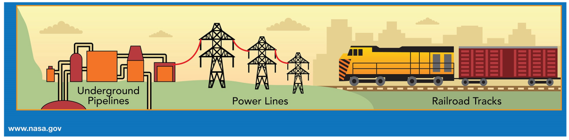
The EMF caused by the solar storm is not measurable if the size of building or even town is considered. It is simply to small, but it can be destructive for any huge metal installation like railway track, pipeline or high voltage transmission power line, see Fig. 1.14. It can for instance destroy anticorrosion system of a pipeline.

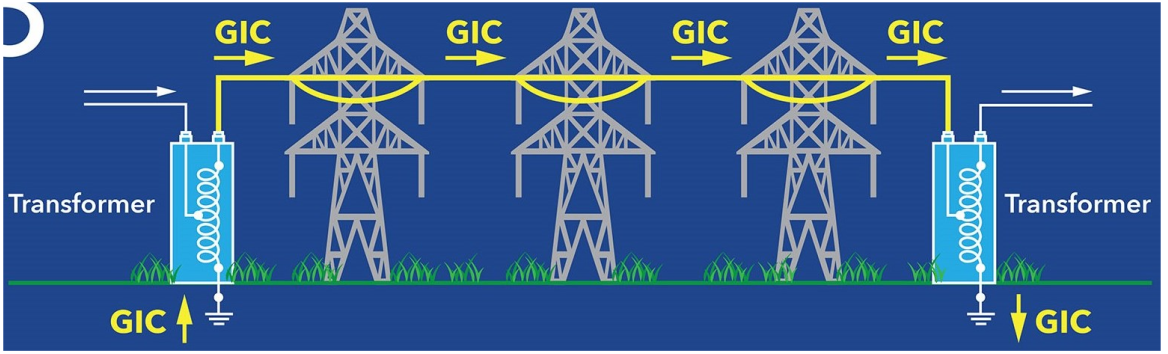
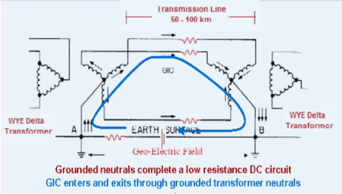
In the North America are operated transcontinental high voltage power transmission lines traced along the parallels of latitude, connecting the east with the west cost. Distances between transformer stations are something like 50 km-100 km. The high voltage pillars have the height of about 30 m. The surface which Earth’s magnetic field is crossing is huge. The star points of the transformers in substations are grounded. This establishes a mesh in which Geomagnetically Induced Current GIC driven by the solar storm EMF can run, see blue line in Fig. 1.15.

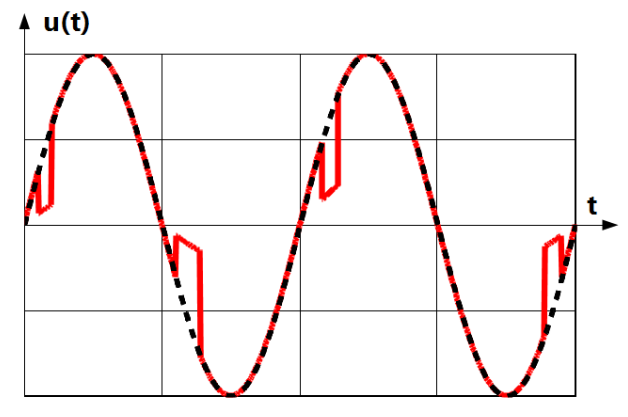
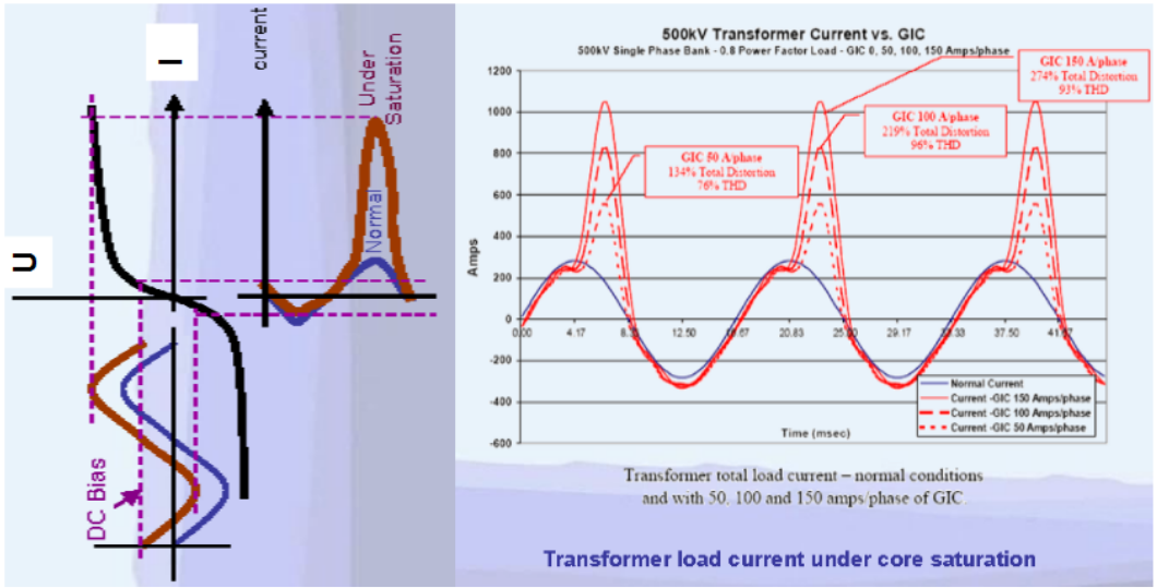
The EMF generated by the solar storm is nearly direct compared to power frequency. Therefore it can be represented as the DC bias overlapped with ordinary operation voltage, see Fig. 1.17. DC bias voltage shits operating point on the [latex]B(H)[/latex] curve² of the transformer core in the substation. In consequence the core saturates for short time segments of the power period. It is mirrored with peaks in transformer current appearing periodically, see Fig. 1.17 causing coils and cores to heat up. In extreme cases, this heat can disable or destroy them, even inducing a chain reaction that can overload transformers and lead to fire of the substation.

Isolating the star point in the substation would make the transmission line much less susceptible to damage due to geomagnetically induced current. However, a transformer that is subjected to this will act as an unbalanced load to the generator, causing negative component current, see Chapter 1.3.2 in the stator and consequently rotor heating.

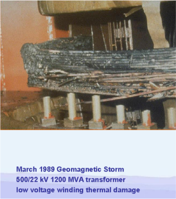
The solar storm in province Quebec in Canada in March 1989 caused power blackout for nine hours. Picture of the transformer winding destroyed by this disaster is shown in Fig. 1.18.

The European grid consists mainly of shorter transmission circuits, which are less vulnerable to damage.