
3 Radio frequency electromagnetic disturbances
Long-term disturbances
Electric discharge in gases
Electrons in metal are free to move around within it. Some of these electrons will have sufficient velocity to escape from the surface of the material. However, when they leave, they produce an electric field which pulls them back to the surface. If an external electric field is present with sufficient field strength, it can overcome the force that normally returns the electron to the surface. The electrons are therefore, removed from the surface and set free.
As electrons finally bombard the anode, the material of anode is heated and may vaporise. In general, either the anode or cathode may vaporise first, depending on the rates at which heat is delivered to and removed form the two contacts. Vaporized metal forms plasma between the electrodes [@Ott] which displaces ions as current’s carrier. Transition from ions’ to plasma’s current takes place in time less than a nanosecond [@Ott].
The filed strength required for initiation of this phenomenon is approximately [latex]500kV/m[/latex] according to [@Ott] and [latex]10 GV/m[/latex] according to [@Clayton]. In Fig.3.2 it is represented with the line with [latex]100 MV/m[/latex] (black continuous line on the left, with black dashed line continuation on the right).
Such big field strength can be generated by small distance of electrodes. Therefore this phenomenon is called short arc. By transition from ions’ to plasma’s current voltage across electrodes drops significantly. To sustain arc minimum arcing voltage and current is required.
After the short arc is initiated the voltage across as well as current through the contact must exceed minimum arcing (sustaining) values. They are dependent on electrodes’ material, as gathered in Tab.3.1, [@Ott].
| Material | Minimum arcing voltage [latex][V][/latex] | Minimum arcing current [latex][mA][/latex] |
|---|---|---|
| Silver | 12 | 400 |
| Gold | 15 | 400 |
| Gold alloy* | 9 | 400 |
| Palladium | 16 | 800 |
| Platinum | 17.5 | 700 |
Short arc can occur even in vacuum, since it does not require the presence of gas. Therefore another name metal-vapor arc. The short arc forms the basis for instance by cutting metals in electro erosion machine tools or in arc welding tools.
If distance between electrodes is to big for initiating short arch discharge, then discharge follows other way which is common also for natural lightning by thunderstorm. Namely, three discharge regimes can be distinguished: dark, glow and long arc. This phenomenon is illustrated in Fig. 3.1 as voltage versus current. Consciously lacks scale of voltage axis in Fig. 3.1 because its quantification depends on type of gas, electrodes’ distance and electrodes’ shape.

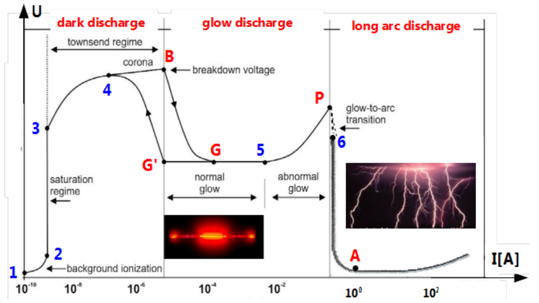
In the region from [latex]1[/latex] to [latex]2[/latex] the background ionisation due to cosmic rays or other sources of ionising radiation takes place. There exist small amount of free electrons and positively charged atoms in gas. Applied voltage accelerates ions. Number of ions does not increase. Some of them, but not all reaches attracting electrode. In point [latex]3[/latex] stream of ions reaching attracting electrode saturates. Range between point [latex]3[/latex] and [latex]4[/latex] means passage to avalanche process. Energy of free electrons is enough for liberating other electrons from electrically neutral atoms by striking them. In consequence number of free electrons and positively charged atoms increases. This is accompanied with emission of electromagnetic energy in form of radio-frequency electromagnetic waves. This is not self sustained process called partial discharge or Ramsauer-Townsend discharge named for its discoverers. Its intensity is proportional to energy of electrons i.e. to the applied voltage. It can cause buzzing on radio receivers. Between [latex]4[/latex] and [latex]B[/latex] emission of electromagnetic energy shifts to visible light. It is called corona discharge which can be observed by high voltage overhead power lines. The same nature has St. Elmo’s fire observable by sailors on top of masts by thunderstorms.
There is hysteresis between [latex]4[/latex] and [latex]G[/latex]. By increased voltage passage follows points [latex]4[/latex], [latex]B[/latex] and [latex]G[/latex], by decreased [latex]G[/latex], [latex]G'[/latex] and [latex]4[/latex]. Between [latex]G[/latex] and [latex]5[/latex] the gas ionization becomes self-sustained.
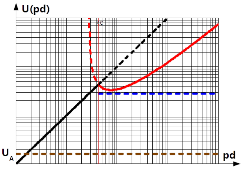
By [latex]B[/latex] amount of ions is such that gas isolation ability ends. Gas starts to glow. This is called breakdown. Paschen found that the breakdown voltage [latex]U_B[/latex] is dependent on the product of electrode separations [latex]d[/latex] and pressure [latex]p[/latex] as
[latex]U_B(p \cdot d) = \frac{K_1 \cdot p \cdot d}{K_2 + \ln{(p \cdot d)}} \label{Paschen_law}\tag{3.16}[/latex]
where [latex]K_1[/latex] and [latex]K_2[/latex] are constants that depend on gas. [latex]\ln{(p \cdot d)}[/latex] is normalised with product of units in which pressure and distance are expressed.
The Paschen curve is shown in Fig.3.2 for air in standard atmospheric pressure as red dashed curve on the left side and solid red curve continuation on the right. Air pressure [latex]p[/latex] and distance [latex]d[/latex] are taken in [latex]Atm[/latex] and [latex]m[/latex] respectively. [latex]K_1 = 43.6\cdot 10^6 / (Atm \cdot m)[/latex] and [latex]K_2 = 12.8[/latex] are applied in Fig.3.2. Minimal breakdown voltage in air by standard atmospheric pressure is approximately [latex]U_B^{min} \approx 320 V[/latex] and occurs at electrodes’ separation [latex]d^{min} \approx 7.6 \mu m[/latex].
Jumping to the self-sustained glow discharge situated on the right to point [latex]G[/latex] is possible, provide the current available from the external circuit exceeds minimum glow discharge sustaining current [latex]I_G[/latex]. Voltage across electrodes drops to
[latex]U_G(d) = 280 + 1000 \cdot d \label{Glow_sust}\tag{3.17}[/latex]
[latex]U_G(d)[/latex] is presented with blue dashed curve in Fig. 3.2.
Voltage drop by transition from [latex]B[/latex] to [latex]G[/latex] is relatively small. In air by atmospheric pressure the breakdown voltage is of order [latex]U_B = 320V[/latex] and glow voltage of order [latex]U_G = 280V[/latex]. Minimum glow sustaining current is quite variable. Its representative range is [latex]I_G \approx 1 - 100 mA[/latex] [@Clayton] Glow regime is utilised in operation of electrical gas lighting equipment.
The voltage across the electrodes [latex]U_G(d)[/latex] for currents between [latex]G[/latex] and [latex]5[/latex] is primarily determined by the dark region between the cathode and the beginning of the glow region, so called the cathode fall region. As the current increases, the dimension of the glow region increases toward anode, but the voltage across the gap remains [latex]U_G(d)[/latex]. In consequence the fall region shrinks and by crossing the threshold field strength for short arc initiation the arcing process starts. State is reached where the heating causes vaporization of the contact metal (point [latex]P[/latex]) resulting in a rapid drop in contact voltage, which marks the beginning of the arc discharge region where in the volume of ionsied gas channels filled with plasma are initiated, point [latex]A[/latex] [@Clayton].
In long arc regime building of channel is completed. Plasma can freely flow between electrodes building conducting bridge. Plasma regime is accompanied with intensive emission of whole spectrum of visible light.
It must be reemphasized that, in order to sustain a glow / arc discharge, the voltage across and current through the contact that are available from the external circuit must exceed [latex]U_G[/latex], [latex]I_G[/latex] and [latex]U_A[/latex], [latex]I_A[/latex] respectively. They are the most left points on the plot in Fig. 3.2.
Actually, plasma current is initiated by long arc discharge identically as by short arc discharge. As it is explained before, voltage fall between electrodes is only in dark, not illuminating segments. In addition by increased current glowing region expands and dark segments shrinks. It means that field strength in dark regions increases leading to heating electrode materials, vaporisation and formation of plasma.
Signals with Amplitude Modulation
Electronic nowadays is predominately digital. It uses variety of modulations for signal transmission. However experience shows, that electronic is mostly susceptible on amplitude modulation AM. That’s why application of AM by most radio frequency EMC immunity tests should be not amazing. Therefore approach to this theme here.
Two waves are combined in AM. One is modulating signal [latex]u_m(t)= m A \cos(2 \pi f_m t)[/latex] in which message is coded and carrier [latex]u_c(t)= A \cos(2 \pi f_0 t)[/latex] responsible for message transportation. [latex]m[/latex] is called modulation depth or modulation index.

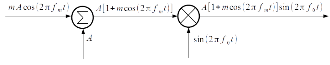
The simplest way of AM, in fact applied in EMC immunity tests is called Double Sideband – Full Carrier DSB-FC. Its principle is explained in Fig.3.3. The modulating signal [latex]u_m(t)[/latex] and amplitude of carrier [latex]A[/latex] are conveyed to the adder. Sum of both signals along with carrier signal are conveyed to multiplier (mixer). Modulated signal at the output of mixer yields
[latex]\begin{array}{rcl} u(t) & = & A \,\sin(2 \pi f_0 t) + mA \, \cos(2 \pi f_m t) \, \sin(2 \pi f_0 t) = \\ & = & \frac{m}{2} \, A \, \sin\left[2 \pi (f_0 - f_m) t \right] + A \, \sin (2 \pi f_0 t) + \frac{m}{2} \, A \, \sin\left[2 \pi (f_0 + f_m) t \right] \end{array} \label{AM-DSB}\tag{3.18}[/latex]

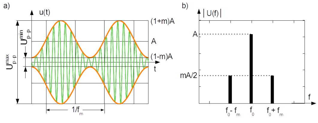
It can be interpreted as the modulated signal (green line in Fig.3.4a)) had been superposition of the pure carrier and carrier with amplitude alternated according to modulating signal, see middle part of Eq.(3.18). Envelope of the instantaneous amplitude of the modulated signal is brown line in Fig.3.4a). In the frequency domain the DSB-FC is represented with three spectral lines, see the right part of Eq.(3.18) and Fig.3.4b).
Obviously RMS of AM DSB-FC signal yields [latex]U_{RMS} = \frac{ A }{\sqrt{2}} \, \sqrt{1 + \frac{m^2}{2}} \label{AM_RMS}\tag{3.19}[/latex]
and consequently power relation of modulated signal [latex]P_m+P_c[/latex] and carrier signal [latex]P_c[/latex]
[latex]\frac{P_m + P_c} {P_c} = 1 + \frac{ m^2}{2 } \label{AM_Power}\tag{3.20}[/latex]
Maximal instantaneous amplitude of the modulated signal is bigger than amplitude of carrier signal by [latex](1+m)[/latex] or about [latex](1+m)dB[/latex] in floating dB. Minimal instantaneous amplitude of the modulated signal is smaller than amplitude of carrier signal by [latex](1-m)[/latex] or about [latex](1-m)dB[/latex] in floating dB.
Maximal instantaneous power of the modulated signal is bigger than power of carrier signal by [latex](1+m)^2[/latex] or about [latex](1+m)dB[/latex] in floating dB. Minimal instantaneous power of the modulated signal is smaller than power of carrier signal by [latex](1-m)^2[/latex] or about [latex](1-m)dB[/latex] in floating dB.
Modulation depth can be easily calculated from the maximal and minimal peak-to-peak spans [latex]U_{p-p}^{max}[/latex] and [latex]U_{p-p}^{min}[/latex] taken from the signal observed in the time domain as shown in Fig.3.4a)
[latex]\begin{array}{rclclrl} \frac{U_{p-p}^{max}}{U_{p-p}^{min}} & = & \frac{ 1+m}{1-m} & \Rightarrow & m & = & \frac{U_{p-p}^{max} - U_{p-p}^{min}}{U_{p-p}^{max} + U_{p-p}^{min}} \end{array} \label{AM_m}\tag{3.21}[/latex]

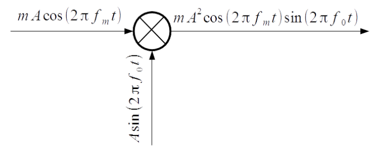
Principle of Double Sideband – Suppressed Carrier DSB-SC is explained in Fig.3.5. The modulating signal [latex]u_m(t)[/latex] and carrier signal [latex]u_c(t)[/latex] are conveyed to multiplier. Modulated signal at the output of it yields

[latex]\begin{array}{rcl} u(t) & = & mA^2 \, \cos(2 \pi f_m t) \sin(2 \pi f_0 t) = \\ & = & \frac{mA^2}{2} \, \sin \left[ 2 \pi (f_0 - f_r) t \right] + \frac{mA^2}{2} \, \sin \left[ 2 \pi (f_0 + f_r) t \right] \end{array} \label{Eq_AM_DSB-SC}\tag{3.22}[/latex]
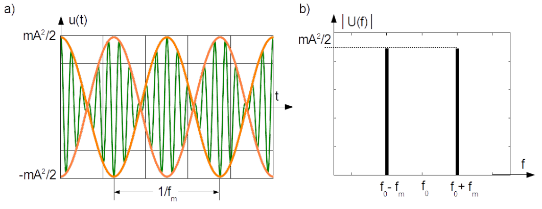
It can be interpreted as the carrier signal (green line in Fig.3.6a)) would have amplitude alternated according to modulating signal, see middle part of Eq.(3.22). Envelope of the instantaneous amplitude of the modulated signal is brown line in Fig.3.6a). In the frequency domain the DSB-SC is represented with two spectral lines, see the right part of Eq.(3.22b) and Fig.3.6b).
There is another amplitude modulation called Single Sideband – Suppressed Carrier SSB-SC. It is realized similarly to DSB-SC with only one difference. Namely low pass or high pass filter is mounted behind the mixer in Fig.3.5. It suppresses either upper or lower spectral line by frequency [latex]f_0+f_m[/latex] or [latex]f_0 - f_m[/latex] respectively.
Sequence of toggled DC voltage
In today’s electronic there are two important branches based on toggling DC voltage. In power electronic, semiconductor valves operating in ON/OFF state are core of appliances such as: AC/AC inverters described in Chapter 3.1, switched mode power supplies SMPS, DC/DC converters, power factor correctors PFC. They are beneficial due to smaller losses and weight and they guarantee flexible, rigid and robust energy sources. In digital, binary electronic logical state 0 and 1 are realized with VOLTAGE/VOLTAGE-LOSS state of the gates.
It is of primary interest to know frequency representation of toggled DC voltage in order to estimate hazards due to side effects of operation of electronic devices.
Rectangular waveform
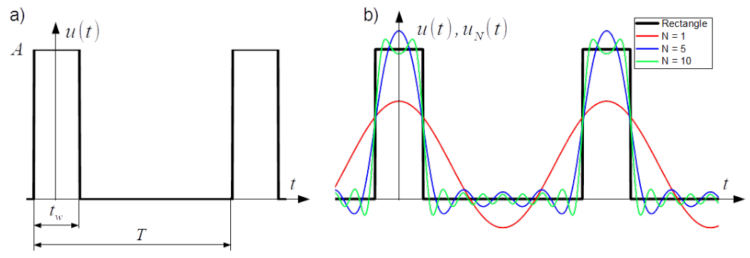
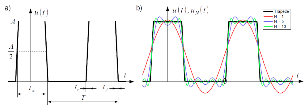
Neglecting the rise and fall time of pulses leads to simplification of toggling which in the time domain is represented with the rectangular waveform as shown in Fig. 3.7 a). Instant [latex]t=0[/latex] in Fig. 3.7 a) coincides with the half of the pulse width [latex]tw[/latex], therefore coefficients [latex]b_n[/latex] in the Fourier series expansion disappears.
Coefficient [latex]a_0 = A t_w/T[/latex] is average value of the waveform. Remaining expansion coefficients [latex]a_n[/latex] are as follows
[latex]a_n = \frac{ 2A}{T} \int_{-\frac{t_w}{2}}^{\frac{t_w}{2}} \cos( n\omega t) dt = 2A \frac{t_w}{T} \frac{\sin\left(n\pi \frac{t_w}{T} \right)}{n\pi \frac{t_w}{T}} \label{Rect_an}\tag{3.23}[/latex]
The pulse width expressed as a ration of the period [latex]t_w/T[/latex], present in Eq.(3.23) is called duty cycle.
Fourier expansion of the rectangular waveform is as follows
[latex]u(t) = A \frac{tw}{T} + 2A \frac{t_w}{T} \sum_{n=1}^{\infty} \left[ \frac{\sin\left(n\pi \frac{t_w}{T} \right)}{n\pi \frac{t_w}{T}} \cos \left(2 \pi n f_1 t \right) \right] \label{u(t)}\tag{3.24}[/latex]
Selected Fourier expansions for [latex]n = 1[/latex], [latex]n = 1, 2, ...,5[/latex] and [latex]n = 1, 2, ...,10[/latex] of the rectangle waveform from Fig. 3.7 a) are presented in Fig. 3.7 b).
Coefficients [latex]a_n[/latex] are values of continuous function [latex]a(f)[/latex] by spot frequencies [latex]f_n = n f_1[/latex], where [latex]f_1 = 1/T[/latex] is fundamental harmonic of the waveform
[latex]a(f) = 2A\frac{ t_w}{T} \frac{\sin\left(\pi t_w f \right)}{\pi t_w f} \label{Envelope1}\tag{3.25}[/latex]
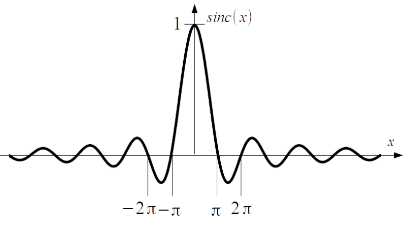
Eqs. from (3.23) to (3.25) encompasses term [latex]\sin x/x[/latex] which is called cardinal sine function [latex]sinc[/latex] and is typical by frequency representation of pulses.
[latex]\mathop{\mathrm{sinc}}(x) = \frac{\sin x}{x} \label{Sinc}\tag{3.26}[/latex]
Function [latex]sinc[/latex] shown in Fig.3.8 is continuous, symmetric, periodic function with period [latex]2\pi[/latex] and value 1 by argument equal to zero, [latex]\mathop{\mathrm{sinc}}(0) = 1[/latex]. It decays to 0 by x approaching plus and minus infinity [latex]\lim_{x \to \pm \infty} \left[\mathop{\mathrm{sinc}}(x) \right] = 0[/latex].

In respect of the harmonics, the lowest frequency of function Eq.(3.25) which must be considered is [latex]f_1[/latex]. Absolute function imposed on [latex]a(f)[/latex] of the waveform from Fig.3.7a) in the frequency range from [latex]f_1[/latex] to infinity is represented with black continuous curve in Fig. 3.9a). It is the envelope of absolute values of the Fourier coefficients [latex]\left|a_n \right|[/latex] for variability of the duty cycles [@Schnorren]. Its downward extrapolation is represented with black dashed line. Notable is its value by [latex]f=0[/latex], [latex]a(0) = 2A\frac{ t_w}{T}[/latex]. It is double value of the [latex]a_0[/latex] of the Fourier expansion. Distinctive are zero cross frequencies which falls by multiple of inverse of the pulse width[latex]1/t_w[/latex]. Notable is the number of harmonics between consecutive zero crossing. It oscillates by reciprocal of the duty cycle. It is four or five for duty cycle equal to [latex]0.23[/latex] as shown in Fig. 3.7 and Fig. 3.9.

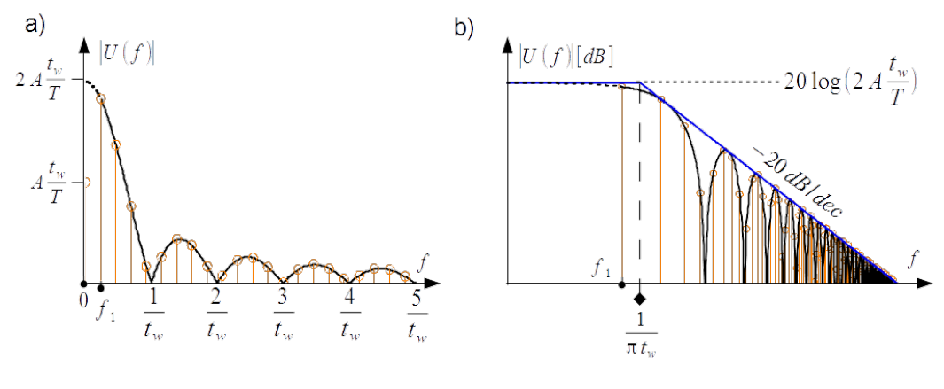
Very practical is representation of the frequency spectrum from Fig. 3.9a) in the double logarithmic scale as shown in Fig. 3.9b). The envelope is as follows
[latex]|U(f)| [dB] = 20 \log{\left( 2A\frac{ t_w}{T}\right)} + 20 \log{\left|\frac{\sin\left(\pi t_w f \right)}{\pi t_w f } \right|} \label{Envelope2}\tag{3.27}[/latex]
For upper bound of the spectrum, [latex]\left|\mathop{\mathrm{sinc}}(\pi t_w f )\right|[/latex] is set to one by low frequencies and [latex]\left|\sin(\pi t_w f )\right|[/latex] is set to one by high frequencies yielding
[latex]|U_p(f)|= \left\{ \begin{array} {ll} 20 \log{\left( 2A\frac{ t_w}{T}\right)} & \text{for}~~f < \frac{1}{\pi t_w } \\ 20 \log{\left( 2A\frac{ t_w}{T}\right)} - 20 \log{\left( \pi t_w f \right)} & \text{for}~~f > \frac{1}{\pi t_w } \end{array} \right. \label{Bounds}\tag{3.33}[/latex]
In consequence the upper bound is composed of two segments of the strait line, horizontal by low frequencies and declined with the slope [latex]-20dB/decade[/latex] by high frequencies, see blue line in Fig.3.9b). The corner frequency depends on the pulse width [latex]1/(\pi t_w)[/latex].
Rectangular modulation, radar pulsing
Trapezoidal waveform
Considered is the case with equal rise and fall time [latex]t_r = t_f[/latex]. Assumption of [latex]t_w = t_{50\%}[/latex] simplifies expression for coefficient [latex]a_0 = A \frac{t_w}{T}[/latex] which is trapeze area divided by the period [latex]T[/latex] i.e. it is average value of the waveform.

Instant [latex]t=0[/latex] in Fig. 3.10 a) coincides with the half of the pulse width [latex]tw[/latex], therefore coefficients [latex]b_n[/latex] in the Fourier series expansion disappears. Remaining expansion coefficients [latex]a_n[/latex] are as follows
[latex]a_n = \frac{ 2A}{T} \left\{ \int_{-\frac{t_w}{2} - t_r}^{\frac{-t_w}{2}} \left[ \frac{1}{t_r} \left(t + t_r + \frac{t_w}{2} \right) \cos(n\omega t) \right] dt + \right. \nonumber[/latex]
[latex]+ \int_{-\frac{t_w}{2}}^{\frac{t_w}{2}} \cos(n\omega t) dt + \nonumber[/latex]
[latex]+ \left. \int_{\frac{t_w}{2}}^{\frac{t_w}{2} +t_r} \left[ \frac{1}{t_r} \left(-t + t_r + \frac{t_w}{2} \right) \cos(n\omega t) \right] dt \right\} = \nonumber[/latex]
[latex]= 2A \frac{t_w}{T} \frac{\sin\left(n\pi \frac{t_w}{T} \right)}{n\pi\frac{t_w}{T}} \frac{\sin\left(n\pi \frac{t_r}{T} \right)}{n\pi\frac{t_r}{T}} \label{Trap_an} \tag{3.29}[/latex]
The [latex]50\%[/latex] pulse width expressed as a ration of the period [latex]t_w/T[/latex], present in Eq.(3.29) is also called duty cycle.
Fourier expansion of the trapezoidal waveform is as follows
[latex]u(t) = A \frac{tw}{T} + 2A \frac{t_w}{T} \sum_{n=1}^{\infty} \left[ \frac{\sin\left(n\pi \frac{t_w}{T} \right)}{n\pi \frac{t_w}{T}} \frac{\sin\left(n\pi \frac{t_r}{T} \right)}{n\pi \frac{t_r}{T}} \cos \left(2 \pi n f_1 t \right) \right] \label{ut(t)}\tag{3.30}[/latex]
Selected Fourier expansions for [latex]n = 1[/latex], [latex]n = 1, 2, ...,5[/latex] and [latex]n = 1, 2, ...,10[/latex] of the trapezoidal waveform from Fig. 3.10 a) are presented in Fig. 3.10 b).
Coefficients [latex]a_n[/latex] are values of continuous function [latex]a(f)[/latex] by spot frequencies [latex]f_n = n f_1[/latex], where [latex]f_1 = 1/T[/latex] is fundamental harmonic of the waveform
[latex]a(f) = 2A\frac{ t_w}{T} \frac{\sin\left(\pi t_w f \right)}{\pi t_w f} \frac{\sin\left(\pi t_r f \right)}{\pi t_r f} \label{TEnvelope1}\tag{3.31}[/latex]
Eq.(3.31) encompasses product of two [latex]sinc[/latex] functions [latex]\mathop{\mathrm{sinc}}\left(\pi t_w f \right)[/latex] and [latex]\mathop{\mathrm{sinc}}\left(\pi t_r f \right)[/latex].
In respect of the harmonics, the lowest frequency of function Eq.(3.31) which must be considered is [latex]f_1[/latex]. Absolute function imposed on [latex]a(f)[/latex] of the waveform from Fig.3.10a) in the frequency range from [latex]f_1[/latex] to infinity is represented with black continuous curve in Fig. 3.11a). It is the envelope of absolute values of the Fourier coefficients [latex]\left|a_n \right|[/latex] for variability of the duty cycles. Its downward extrapolation is represented with black dashed line. Notable is its value by [latex]f=0[/latex], [latex]a(0) = 2A\frac{ t_w}{T}[/latex]. It is double value of the [latex]a_0[/latex] of the Fourier expansion.
Very practical is representation of the frequency spectrum from Fig. 3.11a) in the double logarithmic scale as shown in Fig. 3.11b). The envelope is as follows
[latex]|U(f)| [dB] = 20 \log{\left( 2A\frac{ t_w}{T}\right)} + 20 \log{\left|\frac{\sin\left(\pi t_w f \right)}{\pi t_w f } \right|} + 20 \log{\left|\frac{\sin\left(\pi t_r f \right)}{\pi t_r f } \right|} \label{TEnvelope2}\tag{3.32}[/latex]
For upper bound of the spectrum, [latex]\left|\mathop{\mathrm{sinc}}(\pi t_w f )\right|[/latex] and [latex]\left|\mathop{\mathrm{sinc}}(\pi t_r f )\right|[/latex] are set to one by low frequencies, and [latex]\left|\sin(\pi t_w f )\right|[/latex] and [latex]\left|\sin(\pi t_r f )\right|[/latex] are set to one by high frequencies. In the intermediate frequencies [latex]\left|\mathop{\mathrm{sinc}}(\pi t_r f )\right|[/latex] is set to one and [latex]\left|\sin(\pi t_w f )\right|[/latex] is set to one yielding
[latex]|U_p(f)|= \left\{ \begin{array} {ll} 20 \log{\left( 2A\frac{ t_w}{T}\right)} & for~~f < \frac{1}{\pi t_w } \\ 20 \log{\left( 2A\frac{ t_w}{T}\right)} - 20 \log{\left( \pi t_w f \right)} & for~~\frac{1}{\pi t_w } < f < \frac{1}{\pi t_r } \\ 20 \log{\left( 2A\frac{ t_w}{T}\right)} - 20 \log{\left( \pi t_w f \right)} - 20 \log{\left( \pi t_r f \right)} & for~~f > \frac{1}{\pi t_r[/latex] }
\end{array}
\right.
\label{Bounds}\tag{3.33} $

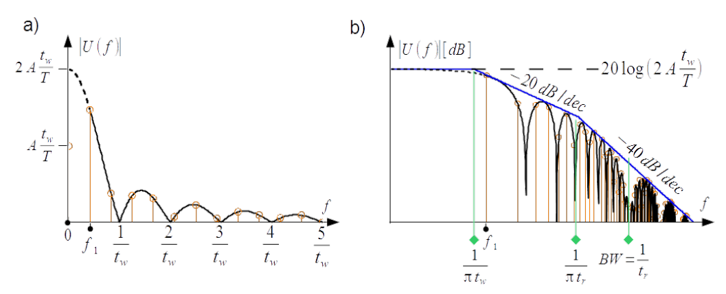
In consequence the upper bound is composed of three segments of the strait line, horizontal by low frequencies, declined with the slope [latex]-20dB/decade[/latex] by intermediate frequencies and declined with the slope [latex]-40dB/decade[/latex] by high frequencies, see blue line in Fig.3.11b). The corner frequencies depends on the pulse width [latex]1/(\pi t_w)[/latex] and the pulse rise time [latex]1/(\pi t_r)[/latex].
Zero cross frequencies marked in and Fig. 3.11a) falls by multiple of inverse of the pulse width [latex]1/t_w[/latex] in the low and intermediate frequencies because term [latex]\left|\mathop{\mathrm{sinc}}(\pi t_r f )\right|[/latex] is negligible. The number of harmonics between consecutive zero crossing in that range oscillates by reciprocal of the duty cycle. It is two or three for duty cycle equal to [latex]0.417[/latex] as shown in Fig. 3.10 and Fig. 3.11.
The frequency bandwidth [latex]BW[/latex] of the trapezoidal waveform defined as follows
[latex]BW = \frac{1}{t_r} \label{BW}\tag{3.34}[/latex]
is marked in Fig. 3.11b). It seems to be very conservative, but if the pulse width approaches the rise time, such bandwidth ensures removal of the spectral lines which approximately are only 27 dB below the fundamental harmonic.
Damped oscillatory waveform
Very ofter happens, that toggled DC voltage is followed with ringing (overshoot/undershoot) due to parasitic inductances and capacitances, for instance in power cable connecting motor with the inverter or in PCB signal path. Analysis of the series RLC circuit supplied with rectangularly switched ON and OFF electromotive force, as shown in Fig.3.12 gives good insight into how this phenomenon is mirrored in the frequency domain.

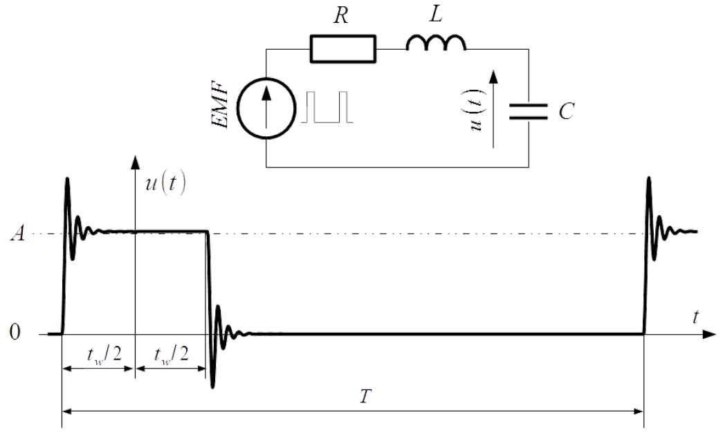

Pattern of damped oscillatory in the period shown in Fig.3.12 is as follows
[latex]u(t)= \left\{ \begin{array} {ll} A - Ke^{-\alpha \left( t+\frac{t_w}{2}\right)} \sin\left[ 2\pi f_r (t+\frac{t_w}{2}) + \varphi \right] & \text{for}~~\frac{-t_w}{2 } < t < \frac{t_w}{2 } \\ Ke^{-\alpha \left( t-\frac{t_w}{2}\right)} \sin\left[ 2\pi f_r (t-\frac{t_w}{2}) + \varphi \right] & \text{for}~~\frac{t_w}{2 } < t < T - \frac{t_w}{2 } \end{array} \right. \label{Ringing_t1}\tag{3.35}[/latex] where [latex]A[/latex] is amplitude of the EMF, [latex]t_w[/latex] is pulse width and [latex]T[/latex] pulse period as shown in Fig.3.12.
The RLC circuit has resonance frequency [latex]f_0[/latex]. By this frequency its impedance is shrunk to resistance [latex]R[/latex]. Damping coefficient [latex]\alpha[/latex] depends on resistance [latex]R[/latex] and inductance [latex]L[/latex].
[latex]\begin{array} {lcr} f_0 = \frac{1}{2\pi} \sqrt{LC} & ; & \alpha = \frac{R}{2L} \label{f0alfa} \end{array}\tag{3.36}[/latex]
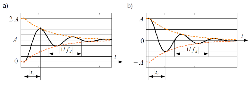
Damped oscillatory frequency [latex]f_d[/latex] is combined with resonance frequency [latex]f_0[/latex] and damping coefficient [latex]\alpha[/latex]. After excitation (step change of EMF in this case) extinguishes, the circuit exhibits damped oscillations with frequency [latex]f_d[/latex], see Fig.3.13. That’s why [latex]f_d[/latex] is called also natural frequency. In that figure the rise time [latex]t_r[/latex] defined as time interval between transient initiation and peak value of the first overshoot is shown.
[latex]K[/latex] depends on amplitude [latex]A[/latex], resonance frequency [latex]f_0[/latex] and natural frequency [latex]f_d[/latex]. [latex]\varphi[/latex] is the phase angle of damped oscillations.
[latex]\begin{array} {lcccr} f_d = \frac{1}{2\pi} \sqrt{4 \pi^2 f_0^2 - \alpha^2} & ; & K = \frac{f_0}{f_d} A & ; & \varphi = \arctan\left( \frac{2\pi f_d}{\alpha} \right) \label{frKfi} \end{array}\tag{3.37}[/latex]

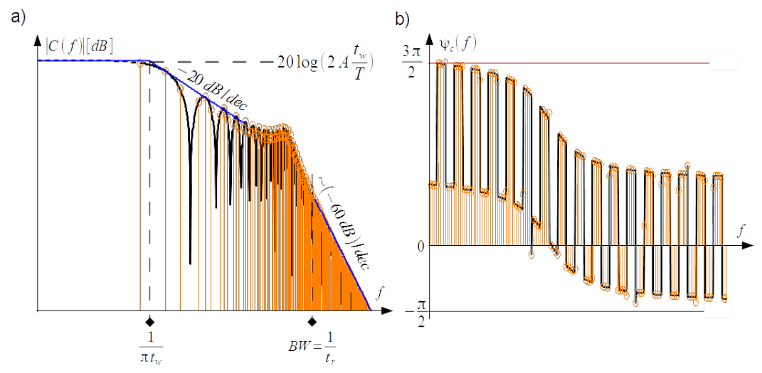
Damped oscillatory as shown in Fig.3.12 is overlapping of three time sequences: rectangle with amplitude A by EMF ON in the time interval [latex][-t_w/2,t_w/2][/latex] and zero by EMF OFF in the time interval [latex][t_w/2,T - t_w/2][/latex], up ringing in the time interval [latex][-t_w/2,t_w/2][/latex], see Fig.3.13a) and down ringing in the time interval [latex][t_w/2,T - t_w/2][/latex] see Fig.3.13b). Therefore coefficients of the Fourier expansion Eq.([an]) and Eq.([bn]) are sums of three integrals. Its complex representation with [latex]C(f)[/latex] as magnitude and phase angle is shown in Fig.3.14.
Upper bound of the spectrum, blue line in Fig.3.14a) are in the lower frequency range the same as for rectangle toggling, i.e. segment of the strait horizontal line up to the corner frequency depending on the pulse width [latex]1/(\pi t_w)[/latex] and line decreased with the slope [latex]-20dB/decade[/latex] above the corner frequency, compare Fig.3.9b).
Remarkable in the spectrum is resonant region in a narrow frequency band. Quality factor and bandwidth of this region depends on [latex]f_0[/latex] and [latex]\alpha[/latex]. Maximum in this region is by ringing frequency [latex]f_r[/latex]. In the case presented here ringing frequency [latex]f_r[/latex] is about forty times bigger than corner frequency and quality of resonance is moderate, therefore maximum of resonance is significantly below the horizontal upper bound. If corner frequency and [latex]f_r[/latex] are closer one to another and resonance has big quality, the resonant region can exceed the upper bound.
Above the resonant region upper bound decays with the slope approximately [latex]\sim (-60dB/decade)[/latex]. Bandwidth frequency defined as usual [latex]BW=1/t_r[/latex] is situated on this slope.

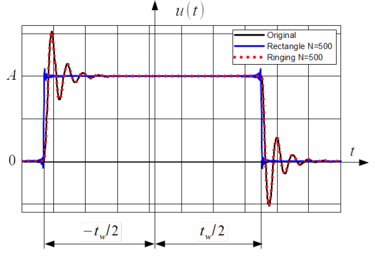
In Fig.3.15 reconstruction of ringing from the frequency domain into the time domain with [latex]N=500[/latex] harmonics (red dotted line) together with the original (black line) ringing is shown. Added is reconstruction of the rectangle (blue line).
Single events - pulses
Spectral density of triangle pulse

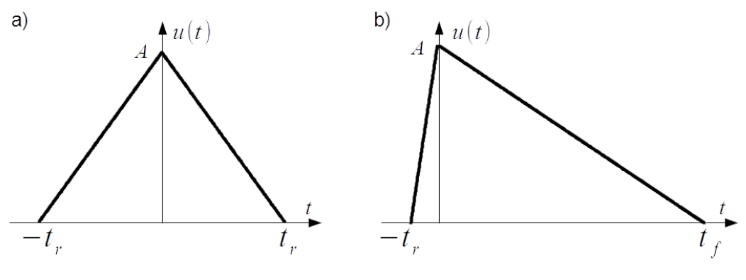
The Fourier integral of the triangle pulse with equal rise and fall time [latex]t_r = t_f[/latex], as shown in Fig.3.16a) according to Eq.([Fourier_int]) yields
[latex]u(f) = At_r \mathop{\mathrm{sinc}}^2\left(\pi t_r f \right) \label{Triangle_tr}\tag{3.38}[/latex]
This spectrum density is a real function with value equal to the pulse area [latex]At_r[/latex] by zero frequency and has zero minima by multiples of the inverse of the pulse rise time [latex]1/t_r[/latex] as shown in Fig.3.17a).

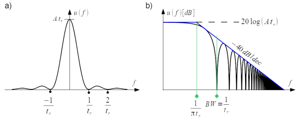
The upper boundary of the spectrum density represented in double logarithmic scale is composed of horizontal line [latex]20 \log\left( At_r \right)[/latex], a slope [latex]-40dB/decade[/latex] and the corner frequency by [latex]f=1/(\pi t_r)[/latex], see Fig.3.17b).
[latex]u_p(f)= \left\{ \begin{array} {ll} 20 \log\left( At_r \right) & \mbox{ for f < \frac{1}{\pi t_r } }\\ 20 \log\left( At_r \right) - 40 \log{\left( \pi t_r f \right)} & \mbox{ for f > \frac{1}{\pi t_r } } \end{array} \right. \label{Bounds_triangle}\tag{3.39}[/latex]
Bandwidth estimation in the same way as for the trapezoidal wave form [latex]BW=1/t_r[/latex] Eq.(3.4), ensures removal of the spectral lines which are approximately 27 dB below the value of spectral density by zero frequency.
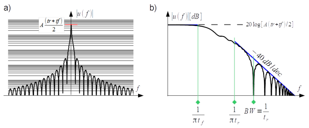
The Fourier integral of the triangle pulse with different rise and fall time [latex]t_r \neq t_f[/latex], as shown in Fig.3.16b) is complex function
[latex]\begin{array} {lcl} Re[u(f)] &= \frac{A}{2 \pi^2 f^2} \left[ \frac{1}{t_r} \sin^2(\pi f t_r) + \frac{1}{t_f} \sin^2(\pi f t_f) \right] = \\ & =\frac{A t_r t_f}{2} \left[ \frac{1}{t_f} \mathop{\mathrm{sinc}}^2(\pi f t_r) + \frac{1}{t_r} \mathop{\mathrm{sinc}}^2(\pi f t_f) \right] \\ Im[u(f)] & = \frac{A}{2 \pi^2 f^2} \left[ \frac{-1}{t_r} \sin(\pi f t_r) \cos(\pi f t_r) + \frac{1}{t_f} \sin(\pi f t_f) \cos(\pi f t_f)\right] \end{array} \label{Triangle_trf_f_Eq} \tag{3.42}[/latex]
It is depicted in Fig.3.18a) in single logarithmic scale in order to accentuate spectrum by high frequencies. This spectrum density is equal to area of the pulse [latex]A(t_r+t_f)/2[/latex] by zero frequency since [latex]\mathop{\mathrm{sinc}}^2(0)=1[/latex].
The upper boundary of the absolute value of the spectrum density represented in double logarithmic scale can be established only by very low and very high frequencies. By very low frequencies imaginary part can be neglecter and the real part builds horizontal line [latex]20 \log\left[ A(t_r+t_f)/2 \right][/latex] as for zero frequency. It ends by corner frequency [latex]1/(\pi t_f)[/latex]. By very high frequencies which starts by another corner frequency [latex]1/(\pi t_r)[/latex] again imaginary part can be neglecter and functions [latex]\sin^2(\pi f t_r)[/latex] and [latex]\sin^2(\pi f t_f)[/latex] in the real part can be replaced with 1. In consequence the upper bound decays with the slope [latex]-40dB/decade[/latex], see Fig.3.18b).
[latex]|u_p(f)|= \left\{ \begin{array} {ll} 20 \log\left( A \frac{t_r + t_f}{2} \right) & \text{for}~~f < \frac{1}{\pi t_f } \\ 20 \log\left[ \frac{A}{2 \pi^2} \left( \frac{1}{t_r} + \frac{1}{t_f} \right)\right] - 40 \log{(f)} & \text{for}~~f > \frac{1}{\pi t_r } \end{array} \right. \label{Bounds_triangle_trf}\tag{3.43}[/latex]

Bandwidth estimation in the same way as for the trapezoidal wave form [latex]BW=1/t_r[/latex] Eq.(3.4), is more conservative than for triangle pulse with equal rise and fall time.
Discharge of static electricity
When two objects rub against each other, some charge (electrons) is transferred from material of one object to material of the other. When these two objects are separated thereafter, this charge may not return to the original one. If the two objects were originally neutral, they are now charged, one positively and the other negatively.
This method of generating static electricity is referred to as the triboelectric effect. Some materials readily absorb electrons while others tend to give them up easily. The triboelectric series is a listing of materials in order of their affinity for giving up electrons [@Ott].
Table 3.2 is a typical triboelectric series. The materials at the top of the table easily give up electrons and therefore acquire a positive charge. The materials at the bottom of the table easily absorb electrons and therefore acquire a negative charge [@Ott].
| : {#Tri | boelectric se | ries} | |
|---|---|---|---|
| 3. | Air | 19. | Sealing wax |
| 3. | Human skin | 20. | Hard rubber |
| 3. | Asbestos | 21. | Mylar |
| 4. | Rabbit fur | 22. | Epoxy glass |
| 5. | Glass | 23. | Nickel, copper |
| 6. | Human hair | 24. | Brass, silver |
| 7. | Mica | 25. | Gold, platinum |
| 8. | Nylon | 26. | Polystyrene foam |
| 9. | Wool | 27. | Acrylic rayon |
| 10. | Fur | 28. | Orlon |
| 11. | Lead | 29. | Polyester |
| 12. | Silk | 30. | Celluloid |
| 13. | Aluminium | 31. | Polyurethane foam |
| 14. | Paper | 32. | Polyethylene |
| 15. | Cotton | 33. | Polypropylene |
| 16. | Wood | 34. | PVC |
| 17. | Steel | 35. | Silicon |
| 18. | Amber | 36. | Teflon |
Amount of energy collected by triboelectric effect depends not only on the ordering of the materials in the series but also on the surface cleanliness, amount of rubbing, surface area in contact, smoothness of surface, the speed of separation and relative humidity [@Ott]. By friction between the blades of the rotor of a helicopter or airfoil of airplane, between isolating wheels and ground floor voltage of static electricity can reach hundreds of kV.
The concern of this lecture notes is human discharge of static electricity which, depending on low/high relative humidity can reach the level of [@Ott]:
- 35 kV / 1.5 kV by walking across carpet,
- 12 kV / 0.25 kV by walking on vinyl floor,
- 6 kV / 0.1 kV worker moving at bench,
- 20 kV / 1.2 kV picking up common polyethylene bag,
- 18 kV / 1.5 kV sitting on chair padded with polyurethane foam.
Different types of human discharge are described in chapter 13 of [@ESD_Ryser], which is contribution of Mr. Heinrich Ryser in the joint publication authored by Mrs. Frank Dittmann, Martin Kahmann.

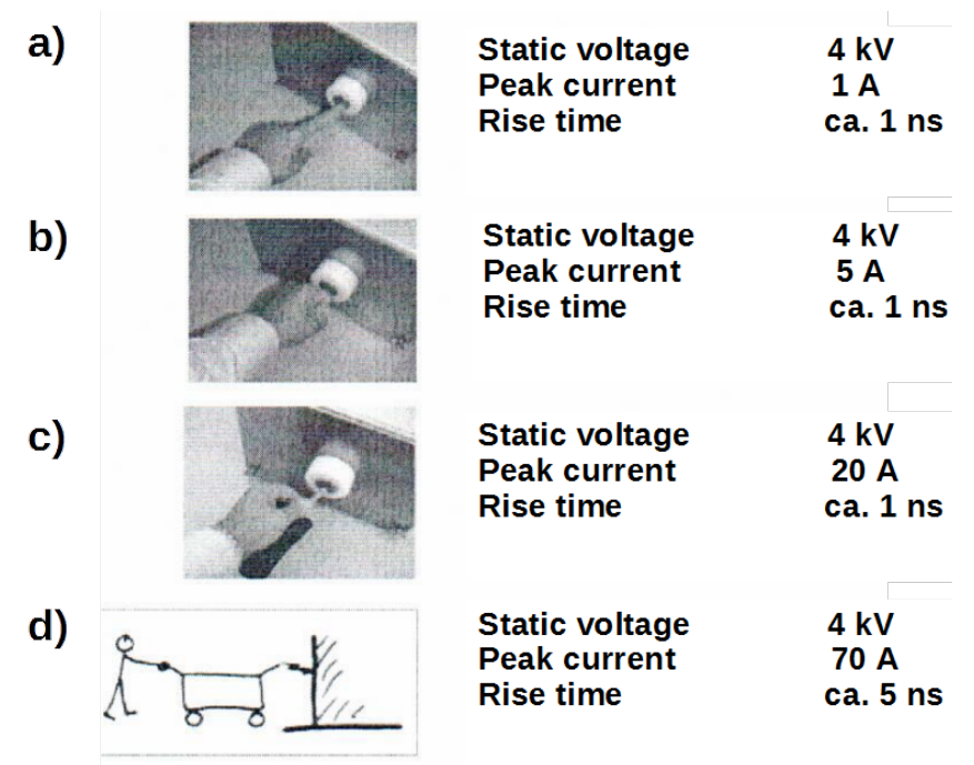
Analysis of Fig.3.19 indicates the human discharge with pointed metal object like: tweezers, key, screw driver or ball pen kept in hand, as most severe discharge. Therefore only this discharge is in scope of standards IEC 61000-4-2 and EN 61000-4-23.

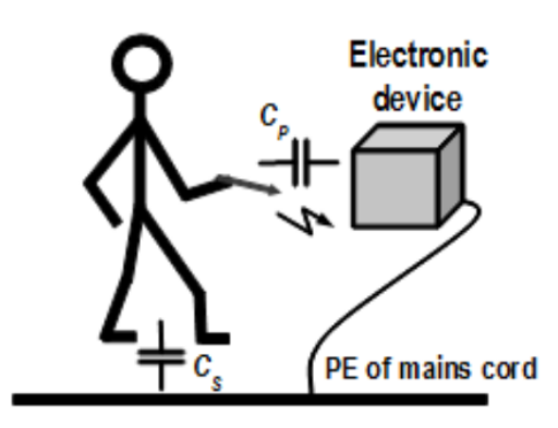
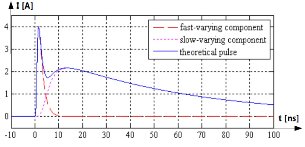
Charged person, standing on the floor can be represented with the charged capacitance [latex]C_P[/latex] of the soles against the ground and the body resistance. If the person is keeping pointed object in hand and approaches grounded electronic equipment [@JB_JSr_TEMC], then electric field strength in small capacitance [latex]C_P[/latex], which by movement of hand is decreased anyway, can exceed value of arc initiation and arc discharge is started. This is the first, fast-varying component of the discharge. The loop is closed and energy stored in capacitance [latex]C_S[/latex] can be dissipated in resistance of human body due to current streaming through the person, arc in capacitance [latex]C_P[/latex], earthing wire in the mains cord and ground. This is the second, slow-varying component of the discharge.
Both components of pulse wave of the human-metal discharge current are shown in Fig.3.21 according to [@JB_JSr_TEMC]. The rise time of the fast component is ca. [latex]800 ps[/latex]. According to Eq.(3.4) it means bandwidth of the ESD up to [latex]1.25 GHz[/latex]. This is the fastest phenomenon in the time domain, discussed in this lecture note and in the same time the widest in the frequency domain.

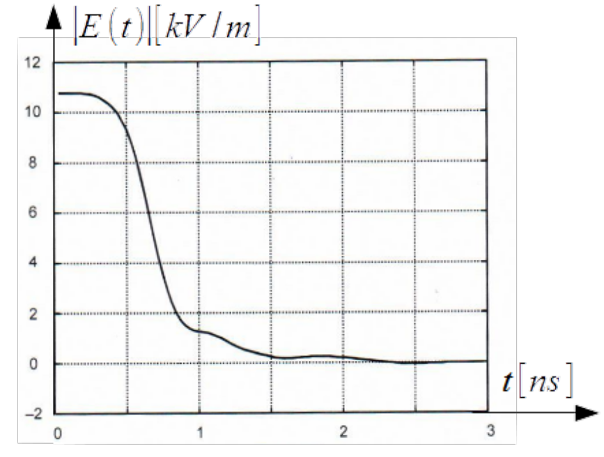
For the sake of completeness module of transient electric field strength [latex]|E(t)|[/latex] of human metal discharge at 5 kV charge voltage and a distance of 10 cm is illustrated in Fig.3.22, according to [@EN-4-2]. The plot is inserted in order to emphasise that although magnetic field and current by discharge of static electricity have pulse form, yet electric field and voltage passes from one to another static state.

Electric fast transients BURST
For explanation of BURST we must return to the chapter 3.1.1. Electric fast transients are generated by opening a mechanical switch in the circuit with inductance. An example is shown in Fig.3.23. Inductance [latex]L[/latex] with serial resistance [latex]R_L[/latex] can represent a choke or motor with conducting losses of winding. In parallel is condenser [latex]C[/latex] covering capacitances between turns. Actually plot of voltage threshold for different discharge regimes in Fig.3.23 is identical as in Fig.3.2 but displayed versus time. It is justified assuming uniform movement of the switch contacts [latex]d=v \cdot t[/latex]. Gas pressure is constant anyway.

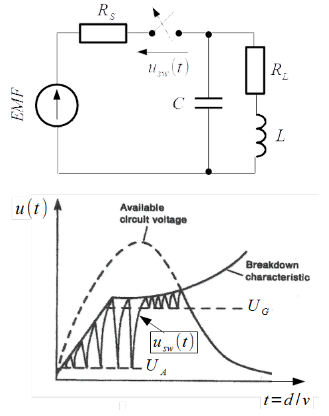
If not any side effect accompanies the opening then the voltage across switch contacts [latex]u_{sw}(t)[/latex] would follow the curve named "available circuit voltage" in Fig.3.23. However shortly after breaking the circuit the field strength between contacts reaches the threshold for short arc initiation. Arc bridges the circuit and voltage across contacts drops rapidly to voltage [latex]U_A[/latex] required for sustaining the arc. Energy stored in capacitance [latex]C[/latex] is dissipated in source resistance [latex]R_S[/latex]. Current through the contacts is usually smaller than minimal sustaining current [latex]I_A[/latex] and arc extinguishes. Voltage across contacts rises up till the field strength between contacts reaches again the threshold for short arc initiation. The next rapid voltage drop on the contacts happens. The repetitive ignition and extinction of arc can continue even in the time after the threshold voltage passes to the Paschen curve (Breakdown characteristic in Fig.3.23), provide voltage across and current through contacts are sufficient for arcing. It means that long arc are generated. Two of them are illustrated in Fig.3.23. Thereafter conditions required for arcing are not fulfilled but fulfilled are conditions for glow discharge. Voltage across contacts drops to voltage [latex]U_G[/latex] required for sustaining the glow discharge. Current through the contacts is usually smaller than minimal sustaining current [latex]I_G[/latex] and glow discharge stops. Voltage across contacts rises up till it reaches again the Paschen curve. The next rapid voltage drop on the contacts happens. These are called miniature burst because jumps between maximal (Paschen curve) and minimal voltage [latex]U_G[/latex] are much smaller. The voltage drops by arcing initiation is as fast as few nanoseconds
Thunderstorm surges
Surges experienced in a building by thunderstorms are implications of direct/close or distant lightning strikes. With direct/close lightning strike are meant the strikes into or in the next vicinity of the: external lightning protection system of the building, case 1 in Fig.3.24, conducting construction of the building like metal windows or facade, into low voltage supply mains or IT network routed into the building case 6.
An example of distant lightning is strike at or next to the medium voltage overhead supply line case 4 or waves traveling in them due to cloud to cloud strike case 5.

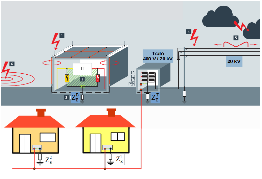
The star point of the low voltage side of the transformer 20 kV/400 V is earthed with an impedance [latex]Z_E^T[/latex], see Fig.3.24. Term earthing impedance is adequate in this context instead of earthing resistance due to dynamics of the event. The 400 V supply line from the transformer to the input of the building has common Neutral [latex]N[/latex] and Protective Earth [latex]PE[/latex] conductor, called [latex]PEN[/latex]. Such supply system is called TN-C. It consists of 4 conductors: [latex]3L,PEN[/latex]. Only at the input to the building [latex]PEN[/latex] is split and laid out as separate Neutral and Protective Earth conductor in the whole building, as so called TN-S supply system with 5 conductors: [latex]3L, N, PE[/latex].
Current driven through the external lightning protection system of the building to earth by direct strike, case 1 in Fig.3.24, causes voltage across earthing impedance [latex]Z_E^B[/latex]. Mind that, the earthing impedance of the building [latex]Z_E^B[/latex], the [latex]PEN[/latex] conductor between building input and the earthing impedance [latex]Z_E^T[/latex] of the transformer along with the earthing impedance [latex]Z_E^T[/latex] of the transformer build the circuit mesh. The current of lightning strike driven in earthing resistance [latex]Z_E^B[/latex] causes surge of voltage across and current driven in the impedance of the [latex]PEN[/latex]. This surge appears automatically in the live conductors of the mains in the whole building. It must be emphasized that voltage and current surge is also present in the earthing impedance of the transformer [latex]Z_E^T[/latex].
Moreover there exists other possible circuit meshes. One of them consists of the earthing impedance of the building [latex]Z_E^B[/latex], the segment of the [latex]PEN[/latex] conductor between building input and the transformer and then either [latex]PEN[/latex] conductor in the supply line of the house 1 and the earthing impedance [latex]Z_E^1[/latex] of the house 1 or the [latex]PEN[/latex] conductor in the supply line of the house 2 and the earthing impedance [latex]Z_E^2[/latex] of the house 2. It means that current driven through the external lightning protection system of the building to earth as shown in Fig.3.24 is sensed as the surge by all customers supplied from the same transformer.
The surge is also sensed everywhere in IT installation due to the fact, that shields of the IT cables are connected to the [latex]PE[/latex] i.e. to the star point in the supply transformer. As already mentioned, the star point of the transformer is also stressed with the surge.
It happen very often that supply mains and IT installation builds loops case 3. Current driven through the external lightning protection system to earth is accompanied with magnetic field. Flux of magnetic field induces voltage surges in them.
Strikes in the medium voltage overhead lines or traveling waves in it can easily get through supply transformer and appear in the building’s mains as a surge.

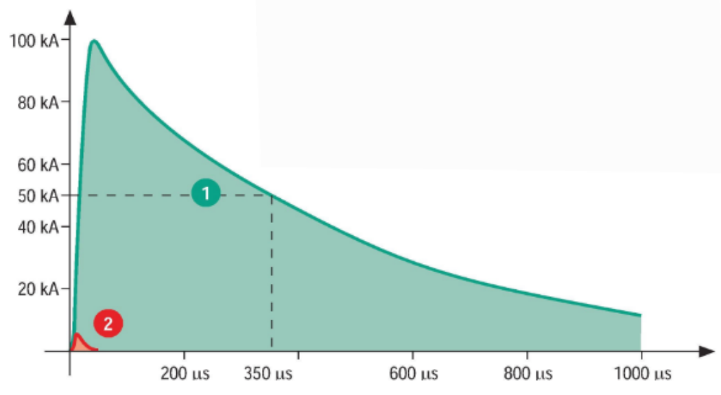
Current by direct strike is a random event. Its parameters like crest (front) time, duration and peak value have statistical distribution. Obviously the same concerns the current surge. These pulses are standardized for objectivity in technical applications. Standardized current pulse by direct strike is defined in the standard [@EN-61643-11] as shown with the plot 1 in Fig.3.25. It is assumed that this current is independent on the load through which it is driven. In other words that energy of the source of this pulse is unlimited.
For comparison, in the same figure standardized current surge defined in the standard [@EN-4-5] is plotted plot 2. Is is assumed that energy of the source of that pulse is limited and the current 2 shown in Fig.3.25 is the short circuit current i.e. current by zero load. Additionally for completeness open circuit voltage of the surge pulse is defined in the standard [@EN-4-5]. Parameters of the direct strike current and surges are gathered in Tab.3.3. In this table the symbol [latex]t_f[/latex] is assigned to the crest time [latex]t_c[/latex] as defined in Fig. [t_r], in order to be in line with the nomenclature of the standard [@EN-4-5].
| Direct strike | |||
| Short circuit | Open circuit | ||
| current | voltage | ||
| Front (crest) time [latex]t_f[/latex] [ [latex]\mu s[/latex] ] | 10 | 8 | 3.2 |
| Pulse duration [latex]t_d[/latex] [ [latex]\mu s[/latex] ] | 350 | 20 | 50 |
| Peak value | 100 [ kA ] | 2 [ kA ] | 4 [ kV ] |
[LEMP_tab]
In Figs. 3.26 and 3.27 standardized surge current and voltage waveforms, according to [@EN-4-5] are shown. They are normalized with the peak value.
It should be noticed that by the short circuit current surge, the rise time [latex]t_r=t_{90\%}-t_{10\%}[/latex] is applied. In consequence relation between the rise and the front (crest) time is as follows [latex]t_f= \frac{100\%}{90\%-10\%} \cdot t_r = 1.25 \cdot t_r[/latex], see Fig.[t_r] and Eq.([t_c]).
For a change by the open circuit voltage surge, the rise time [latex]t_r=t_{90\%}-t_{30\%}[/latex] is applied. In consequence relation between the rise and the front (crest) time is as follows [latex]t_f= \frac{100\%}{90\%-30\%} \cdot t_r \approx 1.67 \cdot t_r[/latex], see Fig.[t_r] and Eq.([t_c]).
As to pulse duration by the short circuit current surge, the pulse width [latex]t_w[/latex] is multiplied with empirical factor [latex]t_d = 1.18 \cdot t_w[/latex] but by the open circuit voltage surge, the time duration is identical with the pulse width [latex]t_d = t_w[/latex]. All these definitions are historically conditioned.

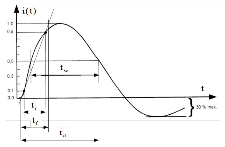

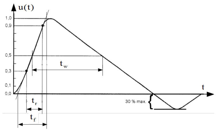
Pay attention to ringing in voltage and current surge, less than [latex]30\%[/latex] as shown in Figs. 3.26 and 3.27. It must be like that because surges are coupled with the direct strike, plot 1 in Fig.3.25 with derive operator.
It can be learned from Tab. 3.3 that the ratio of peak open-circuit output voltage to peak short-circuit current by surge is equal to 2 [latex]\Omega[/latex]. Except unit it has nothing to do with impedance, but nevertheless it is called an effective source impedance in the standard [@EN-4-5].
Nuclear/High-altitude ElectroMagnetic Pulse
After the first experiences with the atomic weapon during the Second World War, the Nuclear Powers started investigation on "humanitarian nuclear weapon" which should be harmless for the human being but paralyzing commandment, logistics and operation of military troops.
Interests were focused on thermonuclear explosions at very high altitude above the Earth in order to avoid the destructive effect of the blast wave and thermal effect. It was expected that ionizing radiations i.e.: [latex]\alpha[/latex], [latex]\beta[/latex], [latex]\gamma[/latex] and neutron radiation by such explosions as well as plasma shell are able to act indirectly on the Earth’s surface in a form of electromagnetic pulse. Thus the term Nucler ElectroMagnetic Pulse NEMP used for indicating this kind of explosions. The outcome of the NEMP on the Earth’s surface is named High-altitude ElectroMagnetic Pulse HEMP.
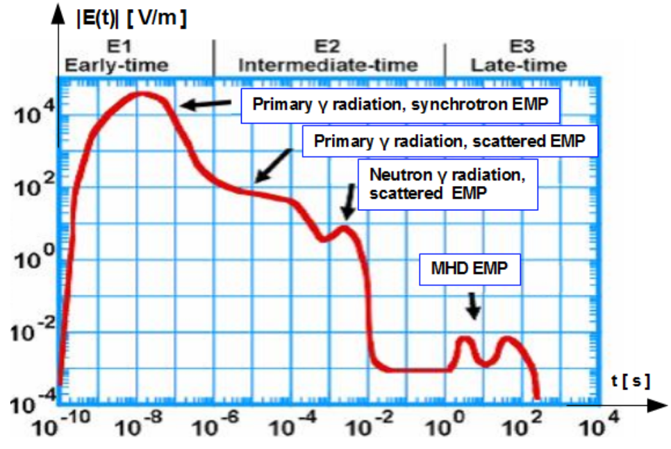
The International Electrotechnical Commission described and standardized the HEMP phenomenon in the document [@IEC-2-9]. Three components of the HEMP namely: E1, E2 and E3 are distinguished there. They are illustrated in Fig.3.28 in the time domain in the double logarithmic scale.

E1 the early time
By thermonuclear explosion at the altitude of several hundreds of kilometers above surface of the Earth i.e. in the ionosphere,4 the primary [latex]\gamma[/latex] rays propagate toward the Earth, as shown in Fig.3.29. Elastic collision of [latex]\gamma[/latex] rays with electrons is ruled with the Compton effect i.e. electrons are accelerated by [latex]\gamma[/latex] rays. As momentum conservation rules this process, the scattered [latex]\gamma[/latex] rays have much smaller frequency shifted to non-ionizing range. Electrons travel generally in downward direction with relativistic speed of more than [latex]90\%[/latex] of the light speed.
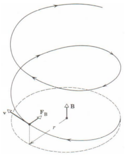
At height between 20 km and 40 km above the Earth’s surface the Earth’s magnetic field comes into play. Magnetic field with induction [latex]\overrightarrow{B}[/latex] exerts a force on electrons moving with the linear speed of [latex]\overrightarrow{v}[/latex]. It is ruled with the Lorenz formula [latex]\overrightarrow{F_B}=e \cdot \overrightarrow{v} \times \overrightarrow{B}[/latex] where [latex]e[/latex] is the charge of electron. By perpendicular orientation of [latex]\overrightarrow{v}[/latex] and [latex]\overrightarrow{B}[/latex] one to another, force [latex]\overrightarrow{F_B}[/latex] would be centripetal and trajectory would be a circle. By other angles the force [latex]\overrightarrow{F_B}[/latex] has also shifting component and the trajectory of electron is helical as shown in Fig.3.30. By the mid latitude electron rotate with the radius of about [latex]85m[/latex].

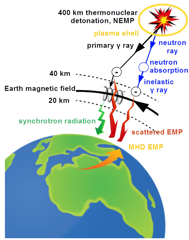
This movement of electrons with linear speed comparable with the light speed and deflected due to angular acceleration is accompanied with the synchrotron electromagnetic radiation like in the synchrotron. This is non ionizing electromagnetic pulse propagating with the speed of light. Standardized E1 pulse has [latex](1.8 - 2.3) ns[/latex] rise time and [latex](23 \pm 5) ns[/latex] half width. I.e. that energy of E1 in concentrated between DC and [latex]1/(\pi \cdot 20ns) \approx 16 MHz[/latex] and pulse bandwidth reaches [latex]BW = 1/(3.05ns) \approx 488MHz[/latex]. Standardized pulse peak value is [latex]50 kV/m[/latex]. Bigger field strength are non realistic due to strongly ionized air. By pure circular movement of electron the field strength of the synchrotron pulse is biggest.

E2 the intermediate time
Scattered [latex]\gamma[/latex] rays, described above is one component of the E2 EMP. Another comes from neutron radiation. Neutron are not able to ionize an atom directly. They can be absorbed by the stable atom. This collision is called inelastic one. By collision atom becomes unstable and is likely to emit the scattered EMP.
E2 has many similarities to thunderstorm lightning, described in chapter 3.3.4 buy it is weaker.
E3 the late time
By thermonuclear explosion so called plasma shell around the source of explosion is build. It is also called plasma ball, light ball or magnetic bubble. It is volume with highly energized plasma which exhibits diamagnetical property. Obviously this bubble deforms the Earth’s magnetic field like solar wind described in chapter 3.4. Moreover the plasma shell spreading toward the Earth comes to the region where is interacts with the Earth’s magnetic field like in the MagnetoHydroDynamic MHD Generator. The Earth’s magnetic field deflects charges of plasma. Positive in one direction, negative in opposite. This evokes strong electric field in the atmosphere oriented horizontally. It is the cause of geomagnetically induced currents in long high voltage power transmission lines and other installations like pipe lines or railroad tracks, as described in chapter 3.4. E3 lasts for about 100 s. It is much shorter than solar storm but it is more intensive.
In 1962 the USA carried out the program of the high altitude nuclear explosions named the Operation Fishbowl. It was launched in July with the 1.44 megaton bomb detonated at the height of [latex]400 km[/latex] above the Johnston Atoll at mid-Pacific Ocean. This experiment had the name the Starfish Prime. Electrical damage in Hawaii, about [latex]1445 km[/latex] away from detonation point were reported. The EMP in Hawaii was relatively weak, about [latex]5.6 kV/m[/latex]. Later calculations showed that if the Starfish Prime had been detonated over the northern continental US, the magnitude of the EMP would have been much larger, [latex]22 kV/m[/latex] to [latex]30 kV/m[/latex] due to greater strength of the Earth magnetic field over the US as well as its different orientation at bigger latitudes.
In the same time Soviet Union performed three high altitude nuclear explosions over Kazakhstan. This program was called Soviet Project K Nuclear Tests. These weapons had only 300 kilotons but at the detonation place the Earth magnetic field is stronger than over the mid-Pacific Ocean. The damage caused by the resulting EMP was much greater than by the Starfish One. The third test called K-3, known also as Test 184 blew fuses and fired all overvoltage protectors in the telephone lines in the radius of [latex]570km[/latex] beneath the detonation point. There were also problems with ceramic insulators on the overhead electric power lines. Current induced in the long underground power line caused a fire in the power plant in the city of Karaganda.
Relevance of the frequency bandwidth BW
In the sections above the frequency bandwidth expressed with the formula [latex]BW = 1/t_r[/latex] is introduced. In [@Clayton] it is asserted that by removal of spectral components above [latex]BW[/latex], the time domain reconstruction of the waveform is marginally distorted from the original one.
This estimate can be interpreted as minimal bandwidth of the low-pass filter which ensures practically undistorted pulse on the filter output. In other words, such filter is transparent for the waveform.
In definition of [latex]BW[/latex] in [@Clayton] the rise time [latex]t_r = t_{100\%-0\%}[/latex] of an ideal pulse is meant. Therefore real pulses verified with the rise time [latex]t_{90\%-10\%}[/latex] must be multiplied by factor [latex]1.25[/latex] according to Eq.([t_c]) and Fig.[t_r] in order to become the crest (front) time [latex]t_c[/latex] which is better estimate of the [latex]t_r = t_{100\%-0\%}[/latex]. It is done so by the ESD, HEMP and BURST pulses in Tab.3.4.
| Phenomenon | Crest (front) time [latex][ns][/latex] | Bandwidth [latex][MHz][/latex] |
|---|---|---|
| ESD | 3.000 | 1’000.000 |
| HEMP, E1 | 3.125 | 320.000 |
| BURST | 6.250 | 160.000 |
| SURGE, open circuit voltage | 1’200.000 | <0.834 |
| SURGE, short circuit current | 8’000.000 | 0.125 |
| LEMP, direct current strike | 10’000.000 | 0.100 |
Mind that oscilloscope is nothing else but low-pass filter. Therefore this definition of the bandwidth gives the hint for choice of the analogue bandwidth of the oscilloscope necessary for trusty recording of the series of pulses or single pulse.