MEASUREMENT OF ACCURACY LIMIT FACTOR OF CURRENT TRANSFORMERS

Introduction

The Current Transformer ( CT) is a type of “instrument transformer” that is designed to produce an alternating current in its secondary winding which is proportional to the current being measured in its primary. The principle of AC CT is based on the magnetic coupling principle. A typical AC CT consists of a toroidal ferromagnetic core, on which a copper wire of N turns is wound. The CT has the bushing, rod type design. The primary winding consists of a firmly built-in aluminium or copper band, the end of which is finished either with a flag-shaped end terminal or with a terminating rod. The secondary winding consists of turns N. A typical AC CT arrangement is shown in Fig. 1.

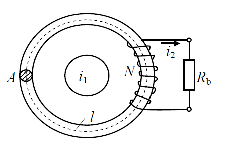
Fig. 1. Basic circuit of the CT

The conductor carrying the measured time-varying current i₁ acts as the primary of the current transformer. The toroid can be clamped around the current-carrying conductor. The winding wound on the toroid acts as the secondary of the current transformer i₂. The burden resistance R_b is selected depending on the sensitivity that is required. For better performance, current transformer cores are desired to have high permeability, high resistivity, low hysteresis and eddy current losses. The cores are made of a high grade ferromagnetic alloys or magnetically oriented transformer sheets. On the outer side of encapsulated core are wound the secondary windings for output currents of 5 A or 1 A. All active parts of transformer are encasted into epoxi resin.

The current transformers are designed for normal operation, it means, the B-H curve dependence of iron core is linear. Under normal operation the difference between primary current i₁ and secondary current i₂ is given by their ratio and the magnetizing current can be neglected. The accuracy of CT in this case is very high, approximately 0.5%.

Different situation is during short circuit conditions in power network, when the primary current of CT is several times higher than under normal operation. It causes the non-linear behavior of the current transformer. As it is known, the DC offset in the fault current following into protective core of current transformer can cause steel to saturate and produce a distorted secondary current. To know exactly a real primary current during fault operation is very important for the correct action of protection relays and also for the analysis focused on faults’ identification and localization. On Fig. 2 the real HV CT was shown.

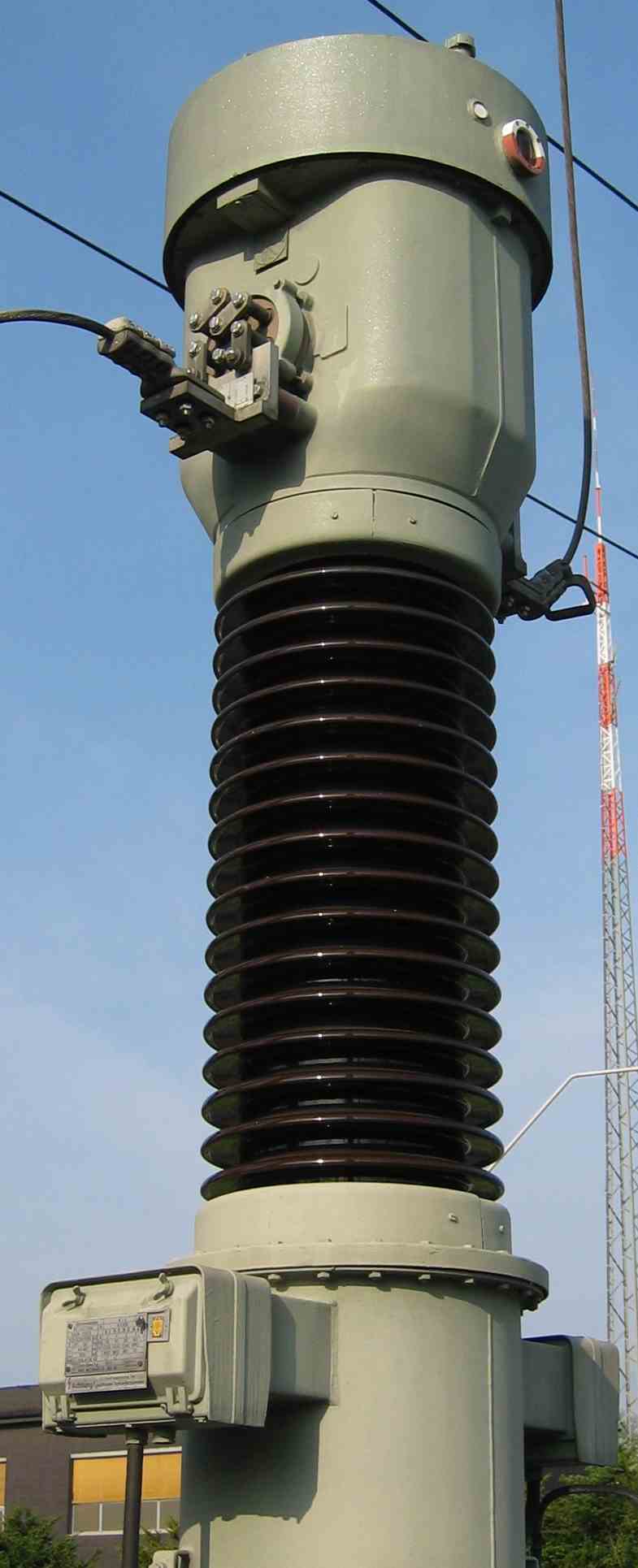
Fig. 2. Example of a real HV CT

Characterication of current transformers

An example of a nameplate of CT and its meaning was shown on Fig. 3. The nominal parameters can be found as:

• rated primary current: 150 A
• rated secondary current: 5 A

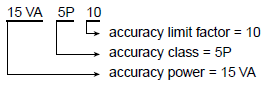
For the protection CT given above, the ratio error is less than 5% at 10 I_n, if the real load consumes 15 VA at I_n.

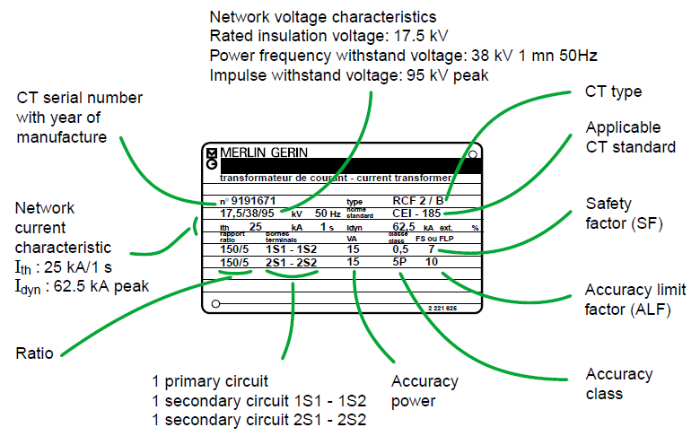
Fig. 3. The example of the nameplate of CT

Accuracy limit ratio n_acr is the ratio of the rated accuracy limit primary current to the rated primary current.

Equivalent circuit diagram and vector diagram

The nonlinear mathematical model of CT can be described in accordance with general equivalent circuit of transformer, but the secondary winding is combined with burden as it can be seen in Fig. 1 and Fig. 4. It consists of lumped parameters of primary winding (resistance of primary winding R₁, leakage inductance of primary winding L₁), secondary winding (resistance R₂, leakage inductance L₂) connected with burden equivalent resistance R_b. In real conditions, R_b is resistance of analogue or digital tester. The lumped parameters of secondary winding are referred to the primary side of transformer. The magnetizing branch is represented by a non-linear magnetizing inductance L_μ, which is a function of magnetizing current I_μ. The eddy current loss is represented by R_FE.

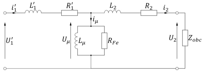
Fig. 4. Equivalent electrical circuit for CT

Vector diagram was shown on Fig. 5, where E₂ = E₁’ represents the electromotive force of CT, which is the same for primary and secondary side. Angles Ψ, φ, δ_i: load impedance angle, angle of the total impedance of the secondary circuit and phase shift between the effective values of the currents I₁’ and I₂. Current I₀’ is a vector characterizing total error of CT, which is equal to magnetizing current I_μ.

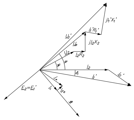
Fig. 5. Vector diagram of CT

Errors of current transformers

For the CTs there can be obtained 3 types of transformation errors:

current error – the error which a current transformer introduces into the measurement of a current and which arises from the fact, that the actual transformation ratio is not equal to the rated transformation ratio

(2)

phase displacement – the difference in phase between the primary and secondary currents, the positive direction of the primary and secondary currents being so chosen that this difference is zero for a perfect transformer

total error ΔI_w – is the RMS value of a current, which is the difference between the instantaneous values of the secondary current multiplied by the rated gear and the values of the primary current, expressed as a percentage of the effective value of the primary current

(3)

Assuming sinusoidal currents, this error can be characterized as, expressed as a percentage, equal to the relative vector value of the difference between the secondary current converted to the primary side and the primary current.

(4)

Characteristics of current transformers

During testing of current transformers, familiarity with the shape of the predicted characteristics is a great help. This allows to take measurements in such a way that the resulting curves faithfully reproduce the actual state. According to the accepted standards, in places where the function significantly changes its value, measurements with smaller changes of regulated parameters should be made, thus causing the density of samples in a given range. The following illustrations show some of the most important charts on current transformers. One of the most important functions is the basic magnetization characteristics of the transformer core (Fig. 6).

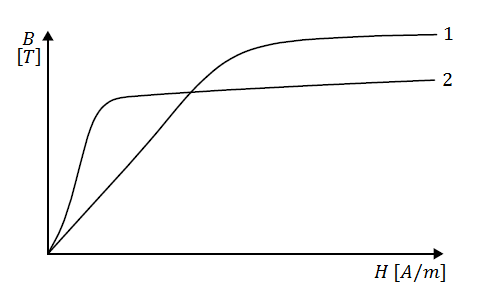
Fig. 6. Basic magnetizing characteristic of a core made of: 1 – Fe and Si; 2 – Fe and Ni

With the change of the Z load impedance the value of the limit of accuracy factor is also changed (Fig. 7). The actual value of the accuracy limit factor corresponding to the load Z₀ is determined by the formula (5).

(5)

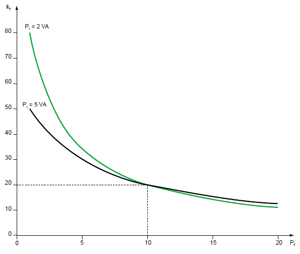
Fig. 7. Behaviour of the accuracy limit factor k_r = f(P_r) of two CTs of 10 VA-5P20 with different internal losses (R_ct) according to the real load connected to the secondary.

Laboratory setup

The laboratory stand is equipped with a set of standard CTs, a test CT, a high-current transformer, an induction regulator and a set of measuring instruments that enable conducting the exercise. The classes of all measuring devices are selected so that the tests are carried out in accordance with the recommendations of the standards.

The measure of accurate limit factor in reality is generally carried out using the direct method by supplying the primary winding with a sinusoidal current. However, if the measurement of this coefficient by the direct method is impossible due to insufficient power source or when there is a risk of damage to the transformer due to overheating during the test, the norms allow the measurement of the accuracy limit factor by indirect methods. However, these methods are acceptable for those transformers for which the internal impedances of a secondary winding measured by one of the known methods at 0.2, 0.5, and 1.2 I_n currents do not differ from each other by more than 10%.

The basic scheme of a stand is shown on Fig. 8. In the laboratory case this scheme was modified. In the place of constant impedance a load box has been placed that allows for step adjustment of the load in the range from 1,25 VA to 125 VA. The power source is a high-current transformer TW powered from the LV network through an RI inductive controller that allows for smooth regulation of the transformer’s power supply voltage

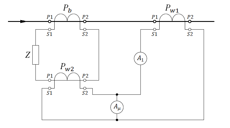
Fig. 8. The basic scheme of a test stand for measuring the accuracy limit factor

In the first step, draw a schematic diagram of the measurement system connections with the gearbox values of the individual current transformers. Next, the correctness of the set gauge gears should be evaluated along with the selection of the appropriate operating ranges. It is recommended to note the rated parameters of the transformers and read the value of the overcurrent currents forced during the tests, at which the tested transformer class is maintained. Before the test is carried out, the team performing the exercise are required to prepare appropriate measurement procedures. The measurement is carried out far beyond the measuring range of the transformer, which causes a significant heating of the transformer core, which forces the user to strive for a maximum short time of testing.

Before starting measurements, the correctness of the test system connections should be verified. Loose connections of wires or current paths should be immediately reported to the instructor. The tests should be performed quickly enough, it usually takes 5 to 8 seconds to set the ammeter readings. The measurement should be made immediately after the ammeter’s readings have stabilized, if the measurement is prolonged, it is allowed to write the results by averaging the values indicated by the ammeter.

The first attempt must be carried out by the teacher who will demonstrate and explain the procedure for taking measurements. Before each subsequent measurement, remember to set the induction controller in the zero position, which is marked on its knob. The measurement starts from the power supply of the test system. It is strictly forbidden to touch the measuring system if the power supply is switched on. Then we increase the output voltage level of the induction regulator by observing the ammeter readings. When the total error is 10%, i.e., when the current I₁ is ten times greater than the current I_μ, the results should be sifted and the system power should be turned off immediately. The Ammeter A₁ should be set to a scale 10 times larger than the A_μ Ammeter, which makes it much easier to carry out measurements that we perform for transformer loads in the range from 30 VA (nominal power value) to 100 VA. The load is changed by means of properly set jumpers of the load box. According to the recommendations, the temperature of the transformer should not exceed 25℃ during measurements, due to the time of the exercise, a minimum deviation from this condition is allowed. The number of measurements should not exceed 5 tests during the entire laboratory. Below is an example table (Table 1) in which the results should be recorded. The last two columns are filled based on the calculations made. The data contained in table 1 allow to sketch the relationship of the limit of accuracy factor to the transformer load value.

Table 1. Basic table for measurements

The given measurement system also allows to plot the dependence of the total error on the value of the transformer’s primary current. The measurement is carried out once at the rated load of the test transformer. By increasing the supply voltage from zero, we read the values of currents I₁, I_μ until the total error is 10%. The measurements are made for the value of the current I₁ with a constant step equal to 0,5 A. Due to the heating of the core, as in the previous tests, the test must be carried out as soon as possible. Reading data can be performed while continuously increasing the supply voltage. Below is an example table (Table 2) in which the obtained results can be saved.

Table 2. Basic table for measurement

Literature

[1] P. Rafajdus, P. Bracinik, V. Hrabovcova, “The Current Transformer Parameters Investigations and Simulations”, Electronics and Electrical Engineering 2010, No. 4 (100)

[2] P. Fonti, Cahier technique np. 194, Current transformers: how to specify them, Merlin Gerin

[3] Instrument Transformers. Application Guide, ABB