Tadeusz Daszczyński; Waldemar Chmielak; and Zbigniew Pochanke

HEATING UP ELECTRICAL DEVICES

Introduction

Reliable operation of electrical power equipment is particularly important from the point of view of continuity of power supply system stability. This also applies to electrical apparatus, each of which has a current path and a contact circuit. Any failure may cause significant material and social losses related to the lack of electricity supply to individual customers. Due to the continuous increase in the values ​​of continuous and short-circuit rated voltages and currents, increasingly high requirements are imposed on current paths as well as on contact systems. Current paths are components of power devices that enable conducting of operating currents. They must be made of conductive materials characterized by high conductivity and high mechanical strength. They are generally made in the form of rigid rails of appropriate shape, cross-section and length, placed specially designed housing. Current paths of electrical apparatus are made primarily of copper, which is the most important conductive material in the power industry. Copper is characterized by very high electrical conductivity. In addition, it is resistant to corrosion. However, these metals have their drawbacks. On the surface of copper and aluminium current paths, layers of compounds may form, which deteriorate the electrical conductivity of the current path in the contacts.

In working conditions, power devices installed in power generation, transmission and distribution systems are loaded in longer time intervals (minutes, hours) with constant values of currents. The devices operating in the circuits of the electric energy receivers can work – depending on the type of the connected receiver in very different load states (Fig. 1a – continuous, 1c – intermittent, 1b – occult, uneven …), at different switching frequencies and different current values.

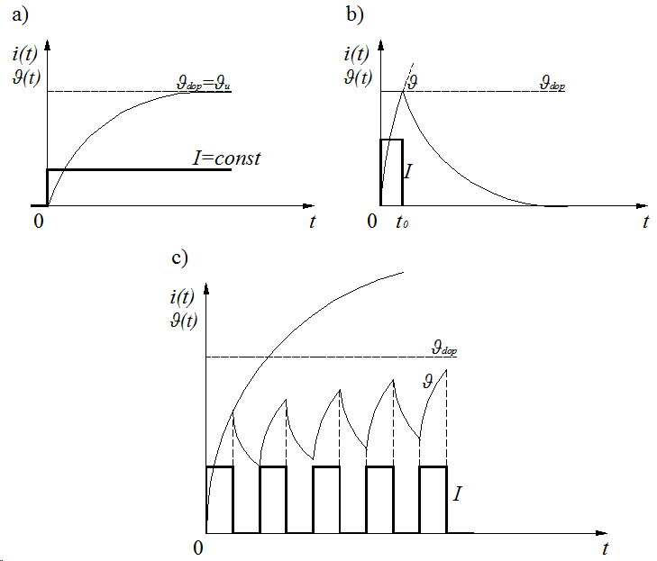
Fig. 1. Different load states for electrical devices

 

The heating of current paths and contacts is an important issue that allows for an accurate analysis of physical phenomena occurring during long-term current flow through the current path. Excessive temperatures of current paths and switching devices contribute to their accelerated degradation and consequently may lead to failure. Current load tests by heating devices testing are among the basic tests required by standards.

 

Joule effect

Energy transformation from electrical current into heat thanks to material resistance to the movement of the electrical charges. In this case, where metal bars are submitted to electrical currents, the power dissipated is equal to (1), considering that neither I or R will change during the experiment (acceptable in our conditions).

 

P = I²R                                                                      (1)

 

Then

(2)

where ρ_elec is the electrical resistivity, L and S are respectively the length and the section of the bar.

The energy dissipated by Joule Effect is of course turned into heat.

 

Thermocouples

The Seebeck Effect (1821):

Thomas Johann Seebeck: When 2 metals are joined at the ends and there a temperature difference between the joints, an electrical potential is generated between the 2 non-joined ends. This magnitude of the voltage is a function of the metal and temperature, this magnitude is in the microvolt range thus a thermocouple can be used to measure either low or high temperatures. The standard configuration is the thermocouple is shown on Fig. 2.

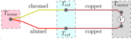
Fig. 2. The standard configuration of thermocouple

The idea is to compare the Seebeck effect generated on each circuit. The circuit composed of chrome and copper will provide a certain potential and the circuit made of aluminium and copper a different one, the difference will be measured by a voltmeter. The contributions of the 2 copper wires are cancelled (same material and same temperature change) so that the voltage measured can be calculated as (3).

 

(3)

Finally it can be obtained the voltage as (4), and the function (5) given by the thermocouple manufacturers.

(4)

(5)

 

 

Labview program

Final Program in LabView is shown on Fig. 3.

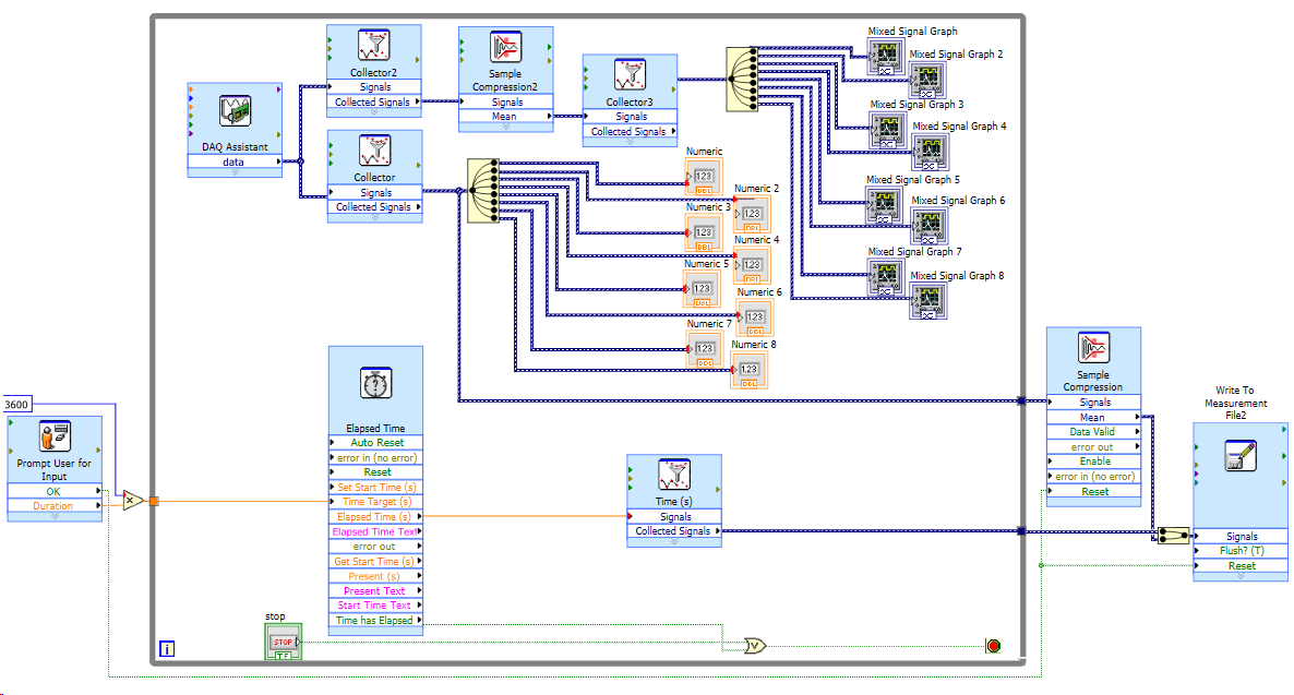
Fig. 3. The LabView program

Laboratory setup

The laboratory setup was built from MV switch NALF 24-6 ABB with nominal parameters:

• Un = 24 kV
• In = 630 A
• Ith = 31,5 kA
• f = 50-60 Hz

This is the indoor switch with fuses. For the experiment, the fuses are shorted using aluminum wires with a rectangular cross-section of dimensions 60×5 mm.

 

Theoretical study:

 

While the program is running and the temperatures of the bars are rising, students will to recover the experimental data by a theoretical approach.

 

– Measure the dimensions of these bars and the current in the bars.

 

– Thanks to these measures, calculate the resistance of the bars and find the powers dissipated by the Joule Effect.

 

Now that the power turned into heat one is able to evaluate the evolution of the temperature in the bars.

 

– Remind the heat equation:

where S is a volumetric heat production.

– On an infinitesimal slice of the bar (dx), what are the incoming and the outgoing heat flux?

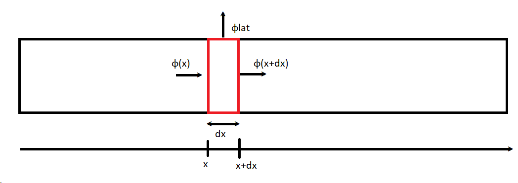
Fig. 4. Conductive bar for explaining the heating up calculations

 

– Perform a balance of all the heat contributions on the slice.

 

 

– Given the fact that the Joule Effect is not localized but volumetric, what can we tell about the temperature along the bar? What conclusions can you draw from this observation?

 

Actually, as the Joule Effect is continuously spread along the bars, the resulting heat is also diffused along these bars, and then the temperature is independent from its position along the bars. This allows us to cancel the flux parallel to the axis of the bars. Then, on our small slice of bar remain the heat production, the flux of heat outgoing by the lateral surface and the difference of temperature on a small time dt.

 

– Right the equation withdrawing the compensating terms,

 

you should obtain this equation:

with

 

– Resolve this 1st order differential equation and compare the result with the experiment.

 

The result is the following one:

with and

 

Which give us the following temperature evolution:

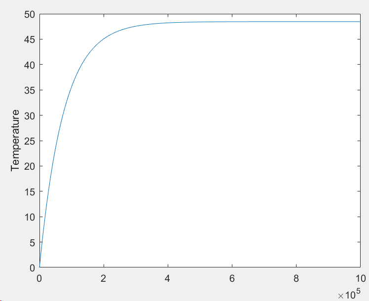
Fig. 5. Evolution of the temperature in a bar in function of time

 

 

 

Electrical Resistivity ρelec:                           Thermic conductance λ:

– Copper: 17E-9 Ω.m                         -Copper: 237 W.m-1.K-1

– Aluminium: 28E-9 Ω.m                   -Aluminium: 280 W.m-1.K-1

 

Thermal Capacity Cp:                                   Density ρ:

– Copper: 385 J.kg-1.K-1                                           – Copper: 8920

– Aluminium 897 J.kg-1.K-1                                – Aluminium: 2700

 

Graphic method for determining the value of a determined temperature increase based on a partial sample

In order to determine the set values of temperature increments Δϑust  individual components of the electrical apparatus can be used with the partial test method. This method is used to determine these values in a situation when during the measurements we did not achieve the determined temperature increments.

The heating curve equation is given by the formula:

where: Δϑ – temperature rise, T – heating time constant.

After differentiation by time it can be found:

As a result of substitution the formula below:

it can be found that:

The final formula for temperature rise become:

The equation of heating up curve is linear function . On the x-axis, when Δϑ = 0, the line describes the section . On the y-axis when  this line describes the section Δϑust, which is the temperature increase one is looking for.

The graphic method for determining the value of a determined temperature increase based on a partial sample is shown on Fig. 6.

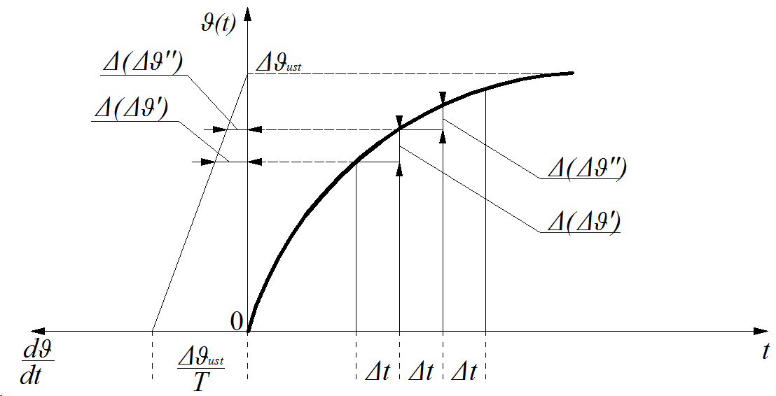
Fig. 6. The graphic method for determining the value of a determined temperature increase based on a partial sample