15 Determination of load flows (fin)
The goal of this laboratory task is to research on the problems of calculating load flows in transmission lines and power transformers. In order to carry out this calculations first it is necessary to create the model of electric power transmission network with preset loads at consuming nodes and preset generations in generating nodes of the network. Load flow calculations are used in the process of electric power system development when new objects such as: lines, transformers and generating units are introduced into service. Everyday exploitation of EPS system operation base on load flow analysis as well. Each change of network topology caused by connection or disconnection of network elements or generating units changes network flows, therefore it is necessary to check on the model the level of load capacity of transmission lines and transformers and also voltage levels.
Models of transmission network elements
The basic transmission network elements are:
- electric power transmission lines,
- power transformers.
Other elements like bus conductors, current and voltage transformers, switches, etc. are treated as non-resistive elements and are not represented in these calculations. In steady state analyses generators with unit transformers are interpreted as the “injections” of power to transmission network.
Model of electric power transmission network
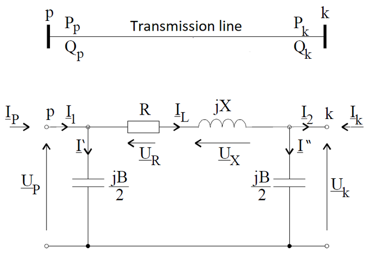
Equivalent scheme of a transmission line connecting two substations – initial p and final k constitutes four-terminal network consisting of resistance R, reactance X and two shunt capacitors of susceptance (inverse of capacitive reactance) B/2.
It is assumed that the specific (per-unit) line electric parameters are given as line catalogue data (nominal data).
So the equivalent scheme parameters of a line are calculated from the following formulae:
R = R’·l;
X = X’·l;
B/2 = B’·l/2;
where: l is the length of the line (km),
R’, resistance (Ω/m),
X’, reactance (Ω/m),
B’/2 susceptance (μS/km)
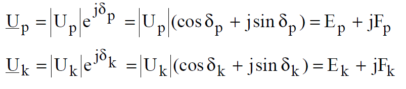
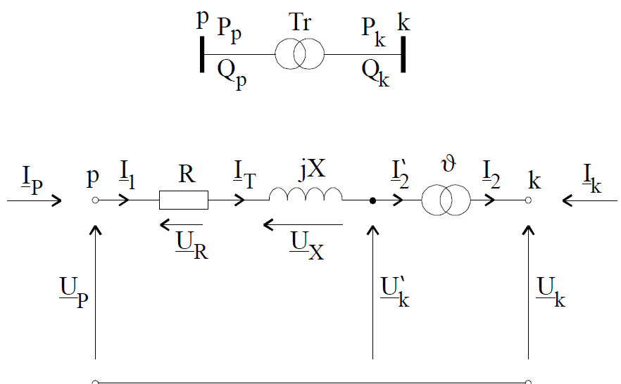
According to electrical engineering laws the values of impedance, alternating currents and voltages and powers in R, L, C circuits are expressed in the category of complex numbers. The task of the methods, algorithms and computational programs is to create such a model of a line, that it would be possible to calculate values of line load (active and reactive powers flowing in Pp, Qp and flowing out Pk, Qk) on the basis of planned operational conditions of such a line. It must be noticed that if the values of voltages Up and Uk on the edges of the line are given (these are complex values):
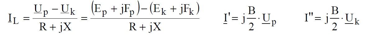
then we can calculate, on the basis of Ohm’s law currents:
and thus the currents flowing in the beginning and in the end of the line (ammeter indications in extreme
substations) are:
Now we can calculate indications of wattmeters:
where ‘*’ is conjugate number.
We should notice that all the formulae regarding the power refer to values in three-phase circuits so there should be √3 present. Because, however, voltages presented in the expressions are phase-to-phase ones, so we do not need to put √3 and then the calculated values of powers are three-phase ones, but the calculated values of currents are √3 times higher than indications of ammeters.
Model of a three-phase power transformer
An electrical power three-phase transformer consists of a core made from ferromagnetic steel sheets on which six windings are wound: three windings on the primary side, connected either in delta or in star, and three windings on the secondary side, suitably connected – in delta or star. For steady state analyses the transmission system transformers are practically modelled by equivalent schemes like in Fig.2. A two-terminal network R, X and an ideal transformer of ratio γ constitute the equivalent scheme of a power transformer for flow calculations.
Impedance parameters (R, X) of a transformer are calculated on the base of measurements performed during the test of the transformer shorting. The experiment consists in that, that one of the windings is shorted and slight voltage is delivered to the other windings (in the order of 10% of rated voltage) such that in these windings nominal current should flow. The ratio of the supplied voltage to the nominal current expresses transformer impedance, and from the measurement of real power released in this case only in transformer windings we can calculate the value of windings resistance. In practice the values of resistance R and reactance X are calculated from parameters given on a transformer rating plate, using the following formulae
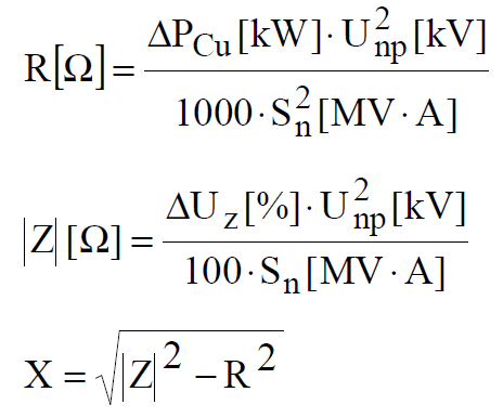
It is not important in calculations on which voltage level (upper or lower) parameters of equivalent scheme will be calculated, we must only consequently define initial and final nodes of the transformer, and impedance and transformation ratio calculate from the side of initial node. Units in which suitable values from rating plate should be substituted in the formulae (5.4) are given in brackets.
It should be underlined that in electrical power calculations performed for transmission networks, the powers are expressed in MVA, MW, Mvar, voltages in kV, currents in kA, and impedance in Ω and impedance reciprocal – admittance is in S (siemens).
Load flows through transformers are calculated similarly like for lines. Assuming that the voltages in the beginning p and in the end k of the transformer are known as complex numbers, we can calculate the current flowing through the transformer:
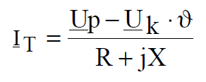
Powers flowing in and flowing out the transformer (wattmeter indications) are:
Vector diagrams
The operation of a transmission network elements (lines, transformers) can be presented on vector diagrams.
A vector diagram, for example for a transmission line, enables to solve graphically the following task: given
voltage |Uk| (voltage module) in the end of the line and the line load Sobc = Pobc+jQobc (real and reactive power
delivered to the final node); calculate voltage in the beginning of the line and current (power) flowing into the
line in its beginning. Exemplary vector diagram of the line is presented in Fig. 3.
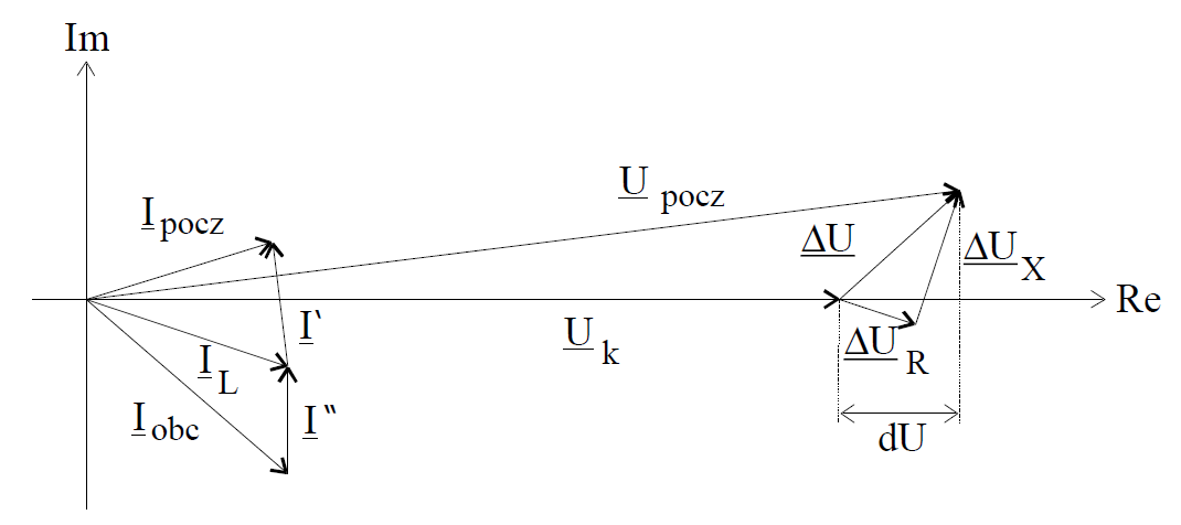
The principles of a vector diagram creation are following:
1. On complex number plane we draw in suitable voltage scale (kV/mm) a vector of the length corresponding
to voltage module preset value in the end of the line. This vector may be drawn at any angle, for example in
the axis of real numbers Re, and its value is:
2. From preset value of line load power Sobc.=Pobc+jQobc. we calculate active and reactive current (at inductive load the current lags the voltage, so the imaginary part Ib in relation (5.8) should be negative, and at capacitive load – positive, leading the voltage):
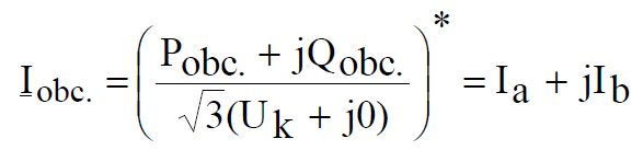
In current scale (A/mm) we draw a vector corresponding to the current vector Iobc (we express currents in amperes).
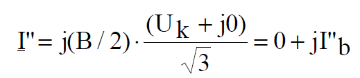
3. From the equivalent scheme of the line (Fig.5.1) it results that to the load current Iobc. we should add capacitive current I” (it should be noticed that in (5.10) the susceptance is expressed in µS, voltage in kV, and the calculated
current should be expressed in A):
4. We add I” to the load current Iobc. and we get current vector in the line IL:
5. We may now calculate voltage ΔUR on the line resistance:
6. Now voltage ΔUX on line reactance is calculated:
7. Vector led out from the origin of co-ordinate system to the end of vector ΔUX is the voltage vector in the beginning of the line – according to Kirchoff’s law it is the sum of vectors:
8. Capacitive current I’ is calculated (similarly like I”) :
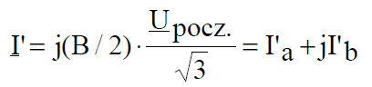
9. Vector drawn from the origin of co-ordinate system to the end of vector I’ is the current vector which flows to the line – according to Kirchoff’s law it is the sum of vectors:
In the vector diagram in Fig.5.3 the following quantities are additionally given:
- voltage drop dU: it is the difference of voltage magnitudes in the beginning and in the end of the line, speaking in other way it is the difference between indications of voltmeters installed in substations in the beginning and in the end of the line; in the vector diagram we should project, for example, voltage vector in the beginning of the line on voltage vector in the end of the line and measure the difference of this projections.
- voltage loss ΔU – it is vector difference (difference of complex numbers) of the voltage in the beginning and in the end of the line; it is a vector (complex number); at the assumed procedure of drawing the vector diagram like in Fig. 3 the numerical value of the real part of voltage loss is equal to the voltage drop.
Transformer vector diagram is drawn similarly as for the line, with exception that in the transformer equivalent scheme the shunt branches usually are not present (Fig.2). After drawing voltage vector of the final node and load current of the transformer they must be reduced to the initial node voltage side – voltage must be multiplied by the ratio, and the current divided. Further procedure is identical like for line vector diagram, with one mentioned exception, that currents I” and I’ are not present.
Model of a transmission network
A mathematical model of an electrical power transmission network it is an admittance model resulting from employing the method of nodal voltages to the solutions of electric circuits. Let simple, exemplary transmission network be given, as in Fig. 4, which task is to lead out the power from two power stations A, D to load substations B, C. The network consists of five transmission 220 kV lines and one 400 kV line connected by two 400/220 kV transformers installed in substations C, D. Arrows directed to the network represent units: generators-transformers in power stations and total flows (injections) of real and reactive power from power stations, and arrows from the network represent network transformers reducing voltage from high (220 kV, 400 kV) to lower (110kV) – total outlets of active and reactive power to the distribution network – loads.
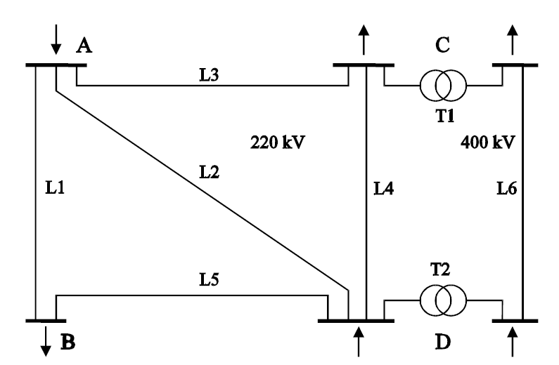
Equivalent scheme of this simple transmission network, created on the basis of line equivalent schemes (Fig. 1) and transformer equivalent schemes (Fig.2) is presented in Fig.5.
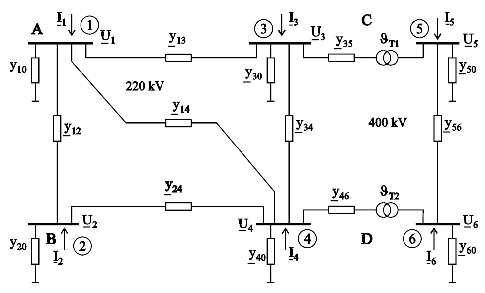
In Fig. 5.5. elements denoted for instance by y12 are the longitudinal branch admittance resulting from reciprocals of series impedance of lines and transformers, and shunt admittance, denoted for example by y10, y20, … result from the values of earth capacities of transmission lines. All admittance are complex numbers and their values are expressed in siemens. Values of nodal voltages, for example U1, U2, … are the values of phase-to-phase voltages on the busses of substations expressed as complex numbers (module and phase angle or real and imaginary part). One of these voltages has imaginary part equal to zero (zero phase angle) – it is a reference voltage. Nodal currents denoted by I1, I2, … they are the current ‘injections’ from sources (generators), and in case of loads they are currents taken by loads with negative sign (they are also complex numbers). Voltages are expressed here in kV and currents in kA. Nodal currents and voltages are presented in the shape of column matrices in order of N x 1, where N is the number of nodes of the transmission network equivalent scheme:
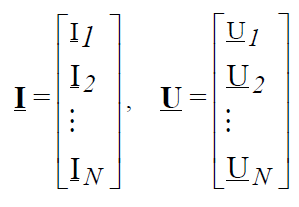
Between nodal voltages U and nodal currents I, according to the nodal voltage method there is the relation:
I = Y*U
where Y is the nodal admittance matrix of dimension N x N, so it has the same number of columns and rows as nodes in the network equivalent scheme. Thus it may be said that each column or row in the admittance matrix represents one node in the network equivalent scheme. In this matrix there are diagonal elements, called committances of the nodes, which are calculated as the sum of all branches connected to the given node. Non diagonal elements are called transadmittances of the nodes and are equal to branches admittance taken with opposite sign – branches connecting directly two nodes. Nodes not connected directly by two branches have transadmittances equal to zero. Admittance matrix is a symmetrical matrix.
Data load flow preparation
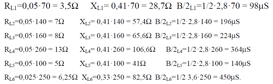
1. Impedance parameters of transmission lines Catalogue data for a transmission line are its length and specific parameters: resistance R’ and reactance X’ in ohm/km and earth capacitance B’ expressed in μS/km. Preparation of data for transmission lines consists in multiplication of specific parameters by the length of the line specified in table.
| Name | R'(ohm/km) | X'(ohm/km) | B’ (μS/km) | Length (km) | Imax |
| L1 | 0,05 | 0,41 | 2,8 | 70 | 780 |
| L2 | 0,05 | 0,41 | 2,8 | 140 | 780 |
| L3 | 0,05 | 0,41 | 2,8 | 160 | 780 |
| L4 | 0,05 | 0,41 | 2,8 | 260 | 950 |
| L5 | 0,05 | 0,41 | 2,8 | 100 | 850 |
| L6 | 0,025 | 0,41 | 2,8 | 250 | 1555 |
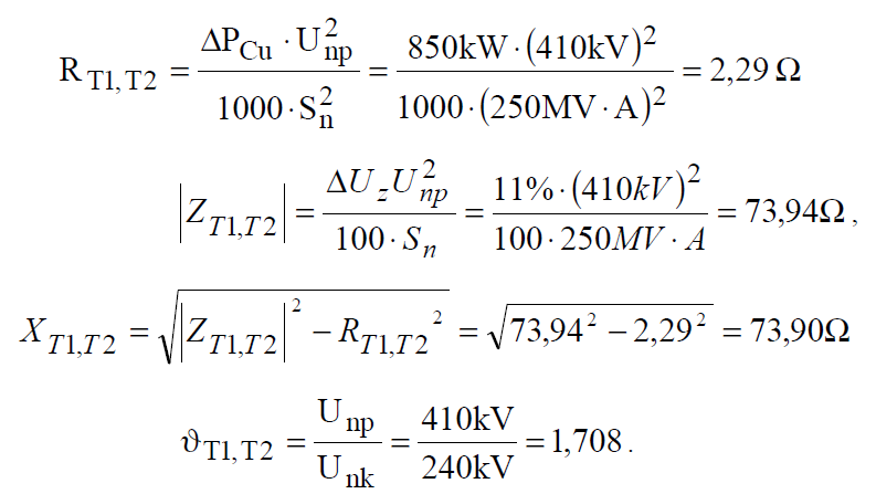
2. Impedance parameters of transformers
Catalogue data for electric power transformers are: nominal power, rated voltage of upper and lower side, real power losses in windings, so called losses in copper and short circuit voltage. On the base of these parameters we can calculate resistance R, reactance X and ratio of the transformer, applying formulae given before. We must choose the initial node of the transformer, for example the initial node may be the node from the upper voltage side, in this case 400 kV and to this voltage we refer transformer resistance and reactance. The choice is arbitrary.
Parameters of transformers T1,T2: Sn = 250 MVA, γ = 410/240 kV/kV, ΔPcu = 850 kW, ΔUz = 11%
Data for calculations by program PLANS are contained in a text file created on a disc of a microcomputer by any text editor. The file with data for the exemplary network is following:
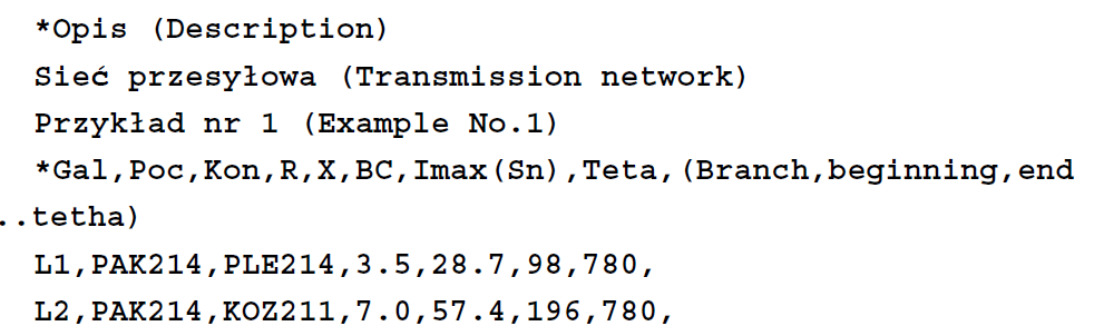
Two basic groups of data should be placed in this file: branch data beginning with the key word *Galezie (all the commands must be in Polish) and nodal data after the key word *Wezly. After the key word *Opis we can put two lines of comment, and in the end of the data it is worth to write the key word *Koniec.
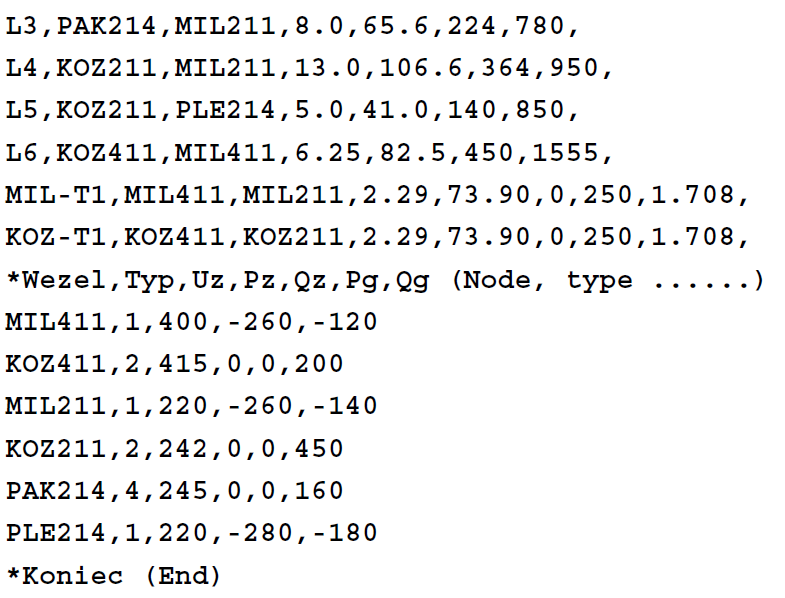
The group of the branch data contains description of one transmission network element in one row. For electric power line we should give: the name of the line, the names of the initial and final nodes, line resistance and reactance and earth capacitance (half), and in the end we can add admissible current of line load. For a transformer 0 should be put in place of earth capacitance and instead of load current – rated power, and after nominal power it is necessary to put transformation ratio. Obviously, as the initial node, there should be written the name of
that node, to which voltage transformer impedance parameters are related.
The group of nodal data consists of records describing individual nodes of transmission network equivalent scheme. One line in the text describes one node and it should contain successively: node name, node type (1,2 or 4), preset or preliminary chosen value of voltage module, active and reactive power drawn from the node (with negative sign) and real and reactive power generated in the node (with positive sign).
After starting the program we should read in the network data to the operational memory by choosing the function Plik->Czytaj dane (File->read data) from the menu. Window for indication the file containing network data will appear on the screen. Exemplary data are in the file named: przyklad.ien (example.ien). The reading in of data is signalled in the computer screen by corresponding information window. The read in network data may be watched and
edited in option: Dane->Węzly (Data->Nodes), Dane->Galęzie (Data->Branches) . After ensuring that the data are correct we can start load flow calculations by choosing the function:
Obliczenia->Rozplywy mocy (Calculations->Load flow).
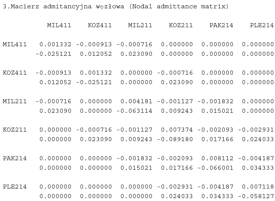
A window will appear on the screen in which all the results of load flow calculations will be presented. The menu of the program will also change. In the group DaneRozplywowe (LoadflowData) there are commands enabling data viewing (Impedancje galęzi and Obciążenia węzlowe) (Branches impedance and Nodal loads). Group Obliczenia (calculations) contains commands enabling performance of calculations. We can determine and watch admittance matrix of network model (Macierz Y) (Matrix Y), nodal power and unbalance in the node (Moc węzla) (Nodal power) and
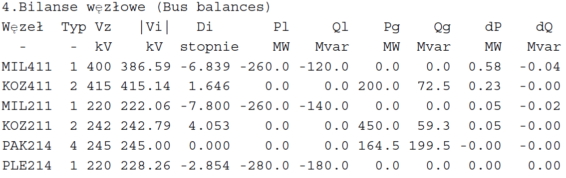
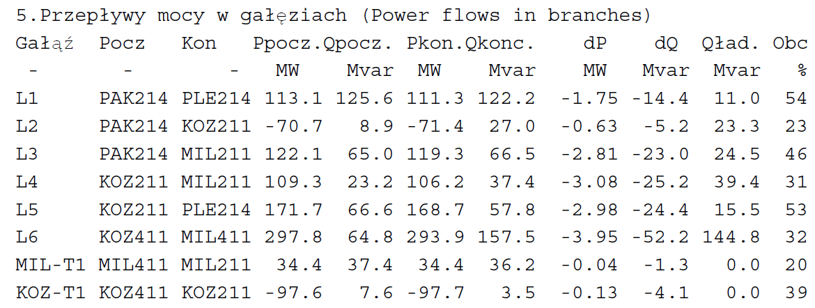
calculation of voltage correction for the chosen node. Choosing the command Rozplyw (Flow) will cause the start of iteration process computing nodal voltages for preset nodal loads – load flow. A window containing information about iteration process will appear. After performing calculations we can watch results choosing Wyniki->Węzly from the menu (nodal voltages) or Wyniki->Galęzie (power flows in lines and transformers). It is the best to perform analyses of the calculated load flow in the graphical mode. To do this we must earlier, with the help of graphical editor of the program Plans, draw the network scheme together with the text description in place of which results of computations will be written in, such as power flows in lines and transformers or nodal powers and voltages. After performance of the iteration process we can start function GrafSym. Menu containing two possibilities will appear on the screen:
Schemat – ready network scheme will be read in from the disc,
Węzeł – choosing a node for graphical analysis in the layout of a network substation scheme.
After choosing the network scheme we should choose the file with the scheme created by the graphical editor from the disc (file with extension *.fgr). After its reading in the figure of the network will appear with the plotted load flow – power flows in lines and transformers and voltage levels in network nodes, and values of powers led in the network and taken from the network – network state of operation on the computer model.
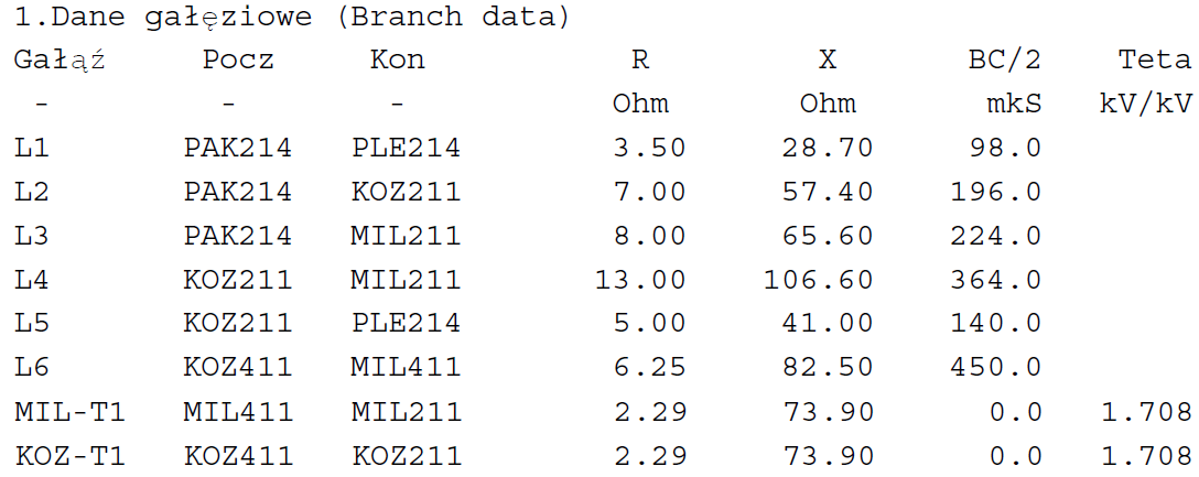
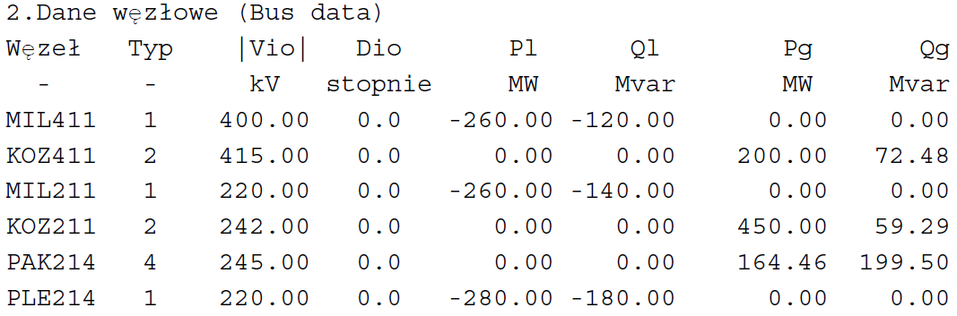
Results of load flow calculations in the form of computer listings received in option “Sprawozdanie” programu Plans (program PLANS report) contain topological and impedance parameters of the transmission network and nodal loads (data for load flow calculations). Then the matrix of committances and transadmittances is printed, and also nodal balances (nodal voltages) and power flows in network branches.
Elaboration of computation results
Test No.: 1
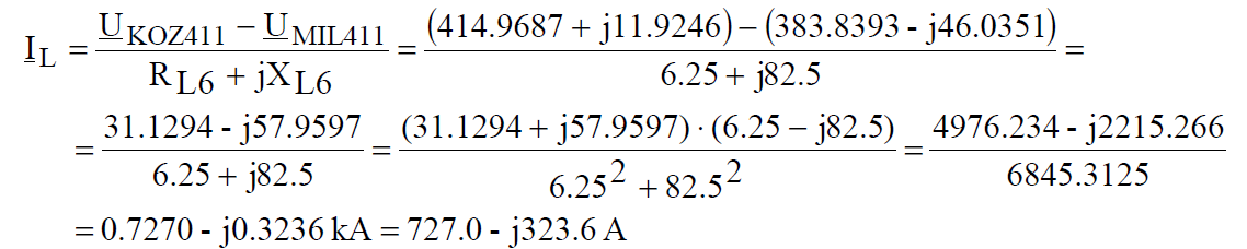
1. Calculate real and reactive power balance in the line:
L6
Given: R,X,B/2 of the line and nodal voltages after iterations.
Calculate real and reactive power flowing in and flowing out of the
electric power line WN, and additionally losses dP=3RI**2,
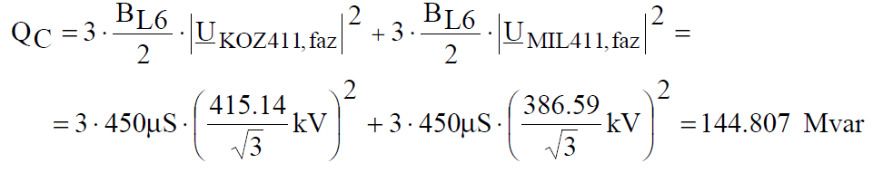
dQ=3XI**2,and charging power QC=BU**2.
Voltages on the edges of the line after iterations:
Current in the line IL:
Line charging currents:
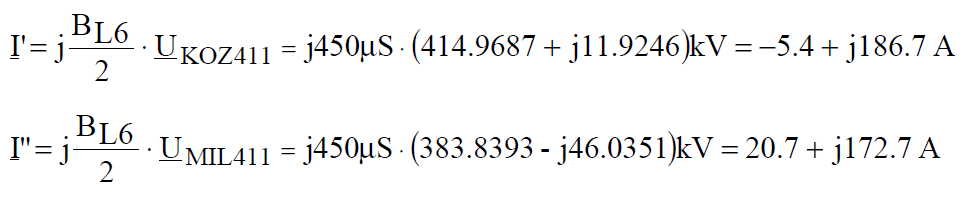
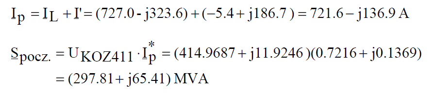
Current and power flowing into the line from bus KOZ411:
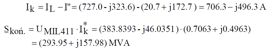
Current and power flowing out of the line at node MIL411:
Active power losses:
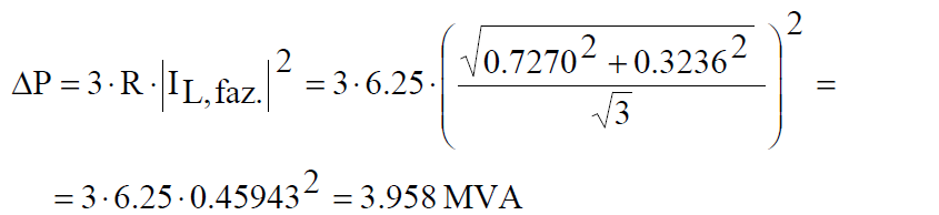
√3 is present in the calculations, because phase-to-phase voltages were taken into account when current was calculated, and because of that previously calculated currents are √3 times higher than correct values – phase currents measured by ammeters.
Reactive power losses:
Line charging power: