
7 Power And Energy
Power and energy in single phase alternating current systems
Electric power system from the point of view of circuit theory is a linear electric circuit of three-phase and single phase sinusoidal current. The three-phase current generated in power plants after the transformation to high voltage is transmitted to customer centers, where after transformation from high to medium voltage and then from medium to low voltage, it supplies single-phase and three-phase receivers. Kirchhoff’s and Ohm’s laws are related to current flows. Characteristic values for AC systems are not only current and voltage, but also power and energy. Electrical power engineers in majority of studies use rather powers than currents, therefore, deciding meaning of voltages and active and reactive power in the calculation of electrical power.
In the simplest case, a single-phase circuit is created by a voltage source loaded by impedance.
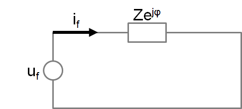
If the instantaneous value of voltage is in the form of:
uf = Ufm sin(wt + yu)
and receivers impedance is: Z = Zejj
then it follows from the Ohm’s law that the instantaneous value of the current is expressed by the formula:
if = Ifm sin(wt + yi) = Ifm sin(wt + yu – j)
where: Ufm, Ifm – voltage and current amplitudes; yi, yu – initial phases of current and voltage, j = yu – yi – phase shift of current and voltage, resulting from impedance loading the source.
The time course of the power results from the product of instantaneous values of voltage and current:
pf = ufif = UfmIfm sin(wt + yu) sin(wt + yi)
Using trigonometric formula:
sina * sinb = 0,5[cos (a – b) – cos (a + b)]
a – b = wt + yu – wt – yi = j
a + b = wt + yu + wt + yi = 2wt + yu + yi = 2wt + 2yu – j
we get the following expression for instantaneous course of the power of the single phase current
pf = 0,5 UfmIfm cosj – 0,5 UfmIfm cos(2wt + 2yu – j)
Effective values of voltage and current Uf and If are related to the amplitudes of these curves using the following equations:
Uf = Ufm/Ö2 If = Ifm/Ö2
Introducing effective values of voltage and current we get the following formula for instantaneous course of the power of the single phase current
pf = UfIf cosj – UfIf cos(2wt + 2yu – j)
From this expression it follows that the instantaneous power oscillates sinusoidally around a constant value
UfIf cosj
with doubled frequency 2f,
The smallest and the largest value of instantaneous power are defined by the equations
pmax = UfIf cosj + UfIf
pmin = UfIf cosj – UfIf
These equations show that, at certain periods of time, the instantaneous power is negative, i.e. the one-phase current flows from the receiver to the AC source. If we assume that the initial phase is
yu = 0
pf = UfIf cosj – UfIf cos(2wt – j)
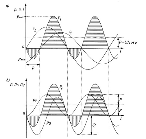
Fig. 1. Courses of instantaneous values of: a) voltage, current and power in a single phase system, b) total power, real power and reactive power in a single phase ac system.
Using trigonometric transformation
cos (a – b) = cosacosb + sinasin b
to the second term, we get
cos(2wt – j) = cos2wt cosj + sin2wt sinj
pf = UfIf cosj – UfIf cos2wt cosj – UfIf sin2wt sinj
pf = UfIf(1 – cos2wt) cosj – UfIf sin2wt sinj
In the above equation we can distinguish two power components, i.e. two courses of the same frequency 2f, but of different amplitudes and average values.
Introducing definitions known from the basic electrical engineering to the equation:
real power as a product of effective values of voltage and current and cosine of the phase shift between voltage and current (power factor)
Pf = UfIf cosj
and reactive power as a product of effective values of voltage and current and sine of the phase shift between voltage and current
Qf = UfIf sinj
simplifies form for the two curves
pf = Pf(1 – cos2wt) – Qf sin2wt
pf = pP + pQ
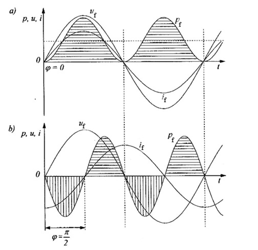
Fig.2. Courses of instantaneous values of: a) voltage, current and power in a single phase system,
b) total power, real power and reactive power in a single phase ac system at load: a) resistive, b) inductive.
Several practical remarks result from this formula:
– Real power Pf is average value of instantaneous power course pf of alternating power, and at the same time it is average value and simultaneously amplitude of the course of component pP , which never reaches negative values
– Physically component pP of the power pulsates with frequency 2f and is responsible for „useful” power send from the source to the load. The value of this power equals real power
Pf = UfIf cos j
Several practical remarks result from this formula:
– Real power Pf depends strongly on the power factor value and for purely resistive load, i.e. cos = 1, the current in the circuit is totally „engaged” in transmission of energy from the source to the receiver
– Reactive power Qf = UfIf sin is equal to the maximum value of the pQ course, i.e. that component of the pf course, which pulsates with the frequency 2f around zero mean value and that is why it does not execute useful work
– In case of reactance connected to the network of alternating current, the mean value of power consumed by the reactance is equal to zero, because the energy transmitted from the source is stored in the reactance (magnetic field of inductivity or electric field of a capacitor). After half of the period it is returned to the source.
Traditionally, inductive reactive power is assumed to be positive and capacitive reactive power is negative. This means that inductance consumes reactive power, but capacity consumes negative reactive power, which often is defined as „generation” of the reactive power by capacity.
The magnetic field energy stored in a coil of inductance L, through which a current of instantaneous value if flows, is defined by the formula:
Wf(L) = 0,5 L Ifm2 sin2(wt + yi)
Using trigonometric formula
sin2α = 0,5(1 – cos2α), we get
Wf(L) = 0,5 LIf2[1 – cos2(wt + yi)]
The energy of magnetic field of a coil is, therefore, sinusoidal function of time with doubled frequency. Every half a period follow oscillations of instantaneous power between the source and the coil.
The energy of electric field stored in a capacitor of capacitance C, on the plates of which an instantaneous voltage has value uf is calculated according to the formula:
Wf(C) = 0,5 C Ufm2 sin2(wt + yu) = 0,5 CUf2[1 – cos2(wt + yu)]
As previously, the energy of electric field of a capacitor is sinusoidal function of time with doubled frequency and every half a period follow oscillations of instantaneous power between the source and the capacitor.
In the analysis of the steady state we often use a complex form of expression of electrical quantities.
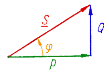
The complex power in an AC system is defined as the vector in a complex space of components corresponding to real power Pf = UfIf cosj and reactive power Qf = UfIf sinj
Sf = Pf + jQf = UfIf cosj +j UfIf sinj
Sf = Sf ejj = UfIf ejj = UfIf ej(yu – yi) = Uf ejyu If e-jyi = UfIf*

Three phase symmetrical source voltages system and three phase symmetrical flowing currents system are assigned to three phase symmetrical system of circuits. On the terminals of a source loaded by a three phase symmetrical receiver
(Z = Zejj in each phase) we have, therefore, the following instantaneous voltages
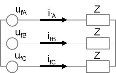
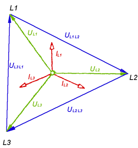
the following instantaneous voltages
ufA = Ufm sin(wt + yu)
ufB = Ufm sin(wt + yu – 120)
ufC = Ufm sin(wt + yu – 240)
(Note that ufA + ufB + ufC = 0)
and the following instantaneous current values
ifA = Ifm sin(wt + yu – j)
ifB = Ifm sin(wt + yu – j – 120)
ifC = Ifm sin(wt + yu – j – 240)
(Note that ifA + ifB + ifC = 0)
In each phase the instantaneous power generated in the source and consumed by the three phase symmetrical receiver is expressed by the formula:
pfA = ufA ifA = Ufm Ifm sin(wt + yu) sin(wt + yu – j)
pfB = ufB ifB = Ufm Ifm sin(wt + yu – 120) sin(wt + yu – j – 120)
pfC = ufA ifA = Ufm Ifm sin(wt + yu – 240) sin(wt + yu – j – 240)
Using trigonometric transformation
sinasinb = 0,5[cos (a – b) – cos (a + b)]
Using trigonometric transformation
sinasinb = 0,5[cos (a – b) – cos (a + b)]
we get in the phase A
a – b = wt + yu – wt – yu + j = j
a + b = wt + yu + wt + yu – j = 2wt + 2yu – j
in the phase B
a – b = wt + yu – 120 – wt – yu + 120 + j = j
a + b = wt + yu – 120 + wt + yu – j – 120= 2wt + 2yu – j – 240
in the phase C
a – b = wt + yu – 240 – wt – yu + 240+ j = j
a + b = wt + yu – 240 + wt + yu – j – 240 = 2wt + 2yu – j – 480
We receive the following formula for the instantaneous course of power in individual phases
pfA = 0,5 UfmIfm cosj – 0,5 UfmIfm cos(2wt + 2yu – j)
pfB = 0,5 UfmIfm cosj – 0,5 UfmIfm cos(2wt + 2yu – j – 240)
pfC = 0,5 UfmIfm cosj – 0,5 UfmIfm cos(2wt + 2yu – j – 480)
Adding instantaneous powers in individual phases we get instantaneous three phase power
p3f = pfA + pfB + pfC = 3 0,5 UfmIfm cosj = 3 UfIf cosj
It results from the last equation that the instantaneous three phase power has constant value, does not pulsate and is equal to the three phase real power or tripled real power of one phase.
Constancy of the instantaneous power in a symmetrical system is a very important feature of the three phase systems. It causes constant torque of three phase turbines and motors, which is measurable and very useful feature. Because the instantaneous three phase power is constant in time, it could seem that the reactive power has no meaning in three phase systems. We should notice, however, that in each phase there is incessant pulsation of power. That is why we introduce the concept of three phase reactive power, analogically to the formula for active power:
Q3f = 3UfIfsinj = 3Qf
From symmetrical treatment of real and reactive power results the formula for complex three phase power and apparent three phase power, which are three times greater than the power in one phase.
S3f = S3fejj = P3f + j Q3f = 3(Pf + jQf) = 3Sfejj = 3Sf
S3f = 3UfIf – apparent three phase power
U = √3Uf I = If
S = 3UfIf* = √3UI* = P + jQ
Both magnetic energy in a symmetrical three phase coil of inductance L and electric energy stored in the three-phase symmetric capacitor of capacitance C have constant value and are defined by the following formula:
Coil
WfA(L) = 0,5 LIf2[1 – cos2(wt + yi)]
WfB(L) = 0,5 LIf2[1 – cos2(wt + yi – 120𗧮 )]
WfC(L) = 0,5 LIf2[1 – cos2(wt + yi – 240𗧮 )]
W3f (L) = 0,5 LIf2[3 – cos2(wt + yi) – cos2(wt + yi – 120𗧮 ) – cos2(wt + yi – 240𗧮 )] =
1/2 LIf2 3 = 3/2 LIf2
Both magnetic energy in a symmetrical three phase coil of inductance L and electric energy stored in a symmetrical three phase capacitor of capacitance C have constant value and are defined by the following formula:
Capacitor
WfA(C) = 0,5 CUf2[1 – cos2(wt + yu)]
WfB(C) = 0,5 CUf2[1 – cos2(wt + yu – 120𗧮)]
WfC(C) = 0,5 CUf2[1 – cos2(wt + yu – 240𗧮)]
W3f (C) = 0,5 CUf2[1 – cos2(wt + yu) – cos2(wt + yu – 120𗧮) – cos2(wt + yu – 240𗧮)] = 3/2 CUf2
Two phase system
ufA = Ufmsin(wt)
ufB = Ufmsin(wt – 180𗧮)
ifA = Ifmsin(wt – j)
ifB = Ifmsin(wt – j – 180𗧮)
pA = UfmIfmsin(wt)sin(wt – j)
pB = UfmIfmsin(wt – 180𗧮)sin(wt – j – 180𗧮)
sinasinb = 0,5[cos (a – b) – cos (a + b)]
in phase A
a – b = wt – wt + j = j
a + b = wt + wt – j = 2wt – j
in phase B
a – b = wt – 180𗧮- wt + j + 180𗧮= j
a + b = wt – 180𗧮+ wt – j – 180𗧮= 2wt – j – 360𗧮
pA = UfmIfmcosj – UfmIfmcos(2wt – j)
pB = UfmIfmcosj – UfmIfmcos(2wt – j – 360𗧮) =
UfmIfmcosj – UfmIfmcos(2wt – j)
p2f = pA + pB = 2UfIFcosj – 2UfIf cos(2wt – j)
p2f = pA + pB = 2UfIFcosj – 2UfIf cos(2wt – j)
In a two phase system the two phase instantaneous power has sometimes negative value, which means that the third conductor is needed for returning of this power from the receiver to the source.
Conclusion: Single phase system needs two conductors to deliver energy, two phase system needs three conductors, the three phase system is the system of the least number of phases which does not need return wire – only three conductors are enough. All the systems with greater number of phases would have the same properties.
Reactive power demand and sources
Reactive power demand in electric power system is caused by the need to create variable magnetic fields in motors, transformers, electric power lines and reactors. As reactive power demand we understand inductive power consumption, which occurs both at energy consumers – mainly in industrial enterprises and at electricity suppliers, it is in the professional power engineering. The flow of current during the transmission of energy causes losses, and because of this active and reactive power led to the network at feed points does not all flow to the customers.
Reactive power demand in electric power system is – with rough approximation – of the same order as real power demand and it periodically changes during a day and a year. The demand is ensured by reactive power sources.
The following sources are used for inductive reactive power generation:
• synchronous generators in electric power plants,
• capacitors for reactive power compensation (connected in parallel),
• controlled reactive power sources – so called FACTS technology elements: SVC and SVG (Statcom),
• synchronous compensators (rarely used – because of high costs),
• synchronous or asynchronous motors (rarely used – because of high costs).
In addition, reactive power is naturally generated by electric power lines because of their capacity. In very high voltage lines the generation of inductive power is very high, and at power flows less than natural power – the loading power is greater than inductive power losses. In overhead lines of rated voltages 750 kV (and greater) compensation of opposite sign is used – permanent shunt reactors are installed (every a few tens of km of the line).
Cable lines generate particularly high inductive reactive power. There exists limited length of a cable line which (uncompensated) would lead only reactive loading power and for active power there would “be lack of cross section” of cable conductors (because of that transmission of power by submarine cables has been for 50 years realized by direct current).
Synchronous generators besides real power produce also reactive power, and the unit costs of reactive power generation in generators are very low. Generators are the cheapest sources of reactive power but only for customers situated close to a power station. With double transformation and transmission over distances of more than several dozen kilometers, reactive power produced in capacitors placed in receiving stations is cheaper. The problem of maintaining bus voltages within acceptable limits and the related problem of proper reactive power management are local problems (in comparison with the actual power flow). Therefore, the transmission of reactive power over long distances is not currently used. Translated with www.DeepL.com/Translator
On the other hand, for technical reasons, it is beneficial to maintain a high (and inductive) power factor cos in power station generating units. Specific and very cheap source of inductive reactive power may be hydro-generators in pumped-storage power plants, which work similarly to large synchronous compensators.
Synchronous compensators, used some time ago, are practically used today due to high costs. They were capable of generating and consuming inductive reactive power (depending on the field current, which can be easily set).
A prerequisite for the cost-effectiveness of synchronous motor operation is the generation of reactive power when the motor is running and not when the motor is running without load. Synchronous motors are rarely used today. Their design is more complex than asynchronous (inductive) motors and their operational characteristics are less suitable for typical applications. In particular, the need to bring them to synchronous rotation during start-up, the need to maintain synchronous rotation and the susceptibility to fall-out of synchronism after exceeding certain torque is – from exploitation point of view – inconvenient.
Static compensators have taken over the role of rotary synchronous compensators – controlled reactive power sources – so-called elements of FACTS technology (flexible AC transmission system): SVC and SVG (Statcom). They have many valuable features, such as the ability to easily adjust the value and sign of compensating power, the ability of application of convenient U = f(Q) regulation characteristics, speed and a series of features not encountered until now. Power electronics elements constitute great part of costs.
These sources are used in high voltage networks (transmission networks) and in medium voltage networks (distribution networks).
Classical capacitors are usually the most economical sources of reactive power. They are used both in very high voltage networks (in this case it is necessary to use matching transformers) and in low voltage networks.
The advantage of capacitors is their low price, very low loss of active power, the possibility of installation at almost any point of the network, easy adjustment of the amount of capacitor battery to the demand for reactive power, simple installation and low workload. Disadvantages of capacitors are: dependence of reactive power generation on voltage square, gradual voltage change during switching on and off, possibility of overload by higher harmonics, high sensitivity to voltage deviations.
Reactive power transmission
Normally active and reactive power sources are situated far from the places of their consumption.
Then the power is transformed many times and sent to the consumers through the network. As it was mentioned – the transmission of reactive power is unprofitable from technical and economical point of view. Power factor cos = P/|S| is a classical index here.
Low power factor in electric power system causes the following disadvantageous phenomena:
Low power factor in electric power system causes the following disadvantageous phenomena:
1. Reduction of generators’ real power capacity prevents them from making full use of their output power. Generator power is limited by the current flowing in armature winding, the driving turbine is fitted to generator real power so to its nominal power factor. Thus if generator works at less than nominal cos – the stator thermal capacity makes it impossible to use the full active power of the unit. Apparent power also decreases at small values of power factor because armature reaction increases, which reduces its electromotive force. This influence may be compensated by the increase of field current, but in such a way that the generator rotor will not be overloaded.
Low power factor in electric power system causes the following disadvantageous phenomena:
2. Reduction of lines and transformers transmission capacity. Transmission capacity is determined by the current causing permissible heating. The flow of reactive power causes necessity of reduction of transmitted real power and this reduction is directly proportional to the power factor. For example, if a transformer with a rated power of 1000 kVA at a power factor of 0.7 can be loaded with actual power of 700 kW, its actual load can be increased to 850 kW with an increase of cos up to 0.85.
Low power factor in electric power system causes the following disadvantageous phenomena:
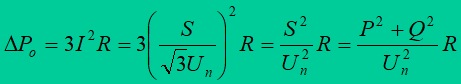
3. Increase of electric energy generation and transmission losses. Active power losses in power system elements depend on the state of load and they increase considerably when receivers power factor decreases. Real power losses are expressed by the formula
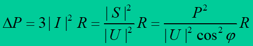
and they are inversely proportional to the square of the power factor
Low power factor in electric power system causes the following disadvantageous phenomena:
4. Increase of voltage drops. If real power P and reactive power Q is transmitted through network element of resistance R and reactance X , then relative voltage drop can be calculated from the formula
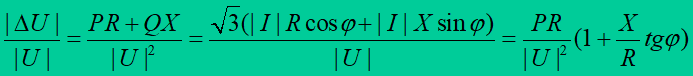
Voltage drop is linearly dependent on tg and the ratio , which is constant value for given network element (G and B shunt – neglected).
For all these reasons, it is very important to improve the power factor in the grid. In the operation of existing network equipment, when loads increase over time and exceed the equipment limit values, in some cases new investments can be avoided by improving the power factor of the receivers.
Using different methods, we are trying to improve the power factor in industrial electrical equipment. Natural ways to improve the energy efficiency of customers should be of primary importance. They do not require the installation of reactive power generation equipment. Once natural resources have been used, a further improvement in cos can be achieved by installing reactive power sources – as already mentioned – most often capacitors.
Natural ways of power factor improvement
In industrial enterprises one can find the following receivers consuming inductive reactive power: asynchronous motors, transformers, driving systems with power electronic elements, electric inductive and arc furnaces, welders, fluorescent lamps, etc.
Analysis of reactive power demand indicates that most reactive power is consumed by asynchronous motors and transformers. So the choice and operation of asynchronous motors has a huge impact on the power factor value and here we have the greatest potential for rationalising reactive power management.
Reactive power drawn by an asynchronous motor may be divided into the following components:
• magnetizing reactive power,
• reactive power losses in motor windings.
The reactive power of magnetization does not depend on the load and is a function of voltage and frequency.
Reactive power losses are proportional to the square of load current and motor fault reactance. They are relatively small and amount to about 10% of the reactive power consumed by the motor at idling speed.
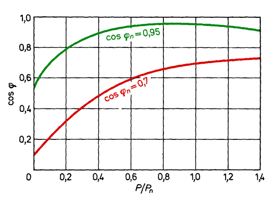
Fig. 6.7. Power factor of an induction motor as a function of its loading (two different motors green and red line)
The power factor value of an asynchronous motor at nominal load depends on rotational velocity, rated power and motor construction. This value changes from about 0.93 (high-speed high power motors) to 0.72 (small low-speed motors). It should be remembered that cos of the engine is not a constant value, but it changes with the change of the engine load, and the lower the actual engine load, the lower the power factor of the engine. The reason for the low power factor in industrial enterprises is, therefore, primarily the operation of motors at loads significantly lower than the rated loads.
So we can list the following natural ways of power factor improvement in industrial enterprises:
1. Proper choice of motor power corresponding to the power of the driven device and selection of the operating mode in such a way that the motors are loaded with more than 70% of the rated power. This guarantees the operation of motors with a power factor close to the nominal.
2. Replacement of durably under-loaded motors by motors of lower power. Under-loaded motor works with reduced power factor and with lower efficiency. On the other hand, the rated efficiency of asynchronous motors decreases with the decrease in their rated power, so it may turn out that after replacing the motor, the reactive power consumption is lower, but the loss of active power is greater; in this case it makes no sense to replace the motors. It is therefore necessary to check whether replacement of engines will reduce the actual power losses in the engine and the mains and to consider whether the additional purchase costs are worth the whole operation. Approximately, it can be said that replacement is advisable if the engine is loaded below 45% of Pn.
3. Shortening the time of motor idle run (and driven devices). Idle run limitation brings doubled advantage: real power losses and drawn reactive power decrease. Idle run may be caused by improper service or the character of technologic process. Eventually idle run limiters may be used. Application of limiters is purposeful, when the consumption of energy for start-up is lower than the energy taken at idle run and when the frequent start-up does not overheat the motor. Normally we assume that the motors can be switched-off if the idle run lasts longer than 10 seconds.
5. Use of synchronous motors, for example, in ventilator drives, compressors, water pumps, etc.
6. Proper maintenance and conservation of motors. Improperly done repair causes reduction of efficiency and power factor. The size of air gap and number of turns have vary great influence on reactive power consumed by asynchronous motor. Enlargement of the gap through axial movement or decreasing the number of turns during rewinding causes significant rise of magnetizing current, which is followed by decrease of nominal power factor.
7. Application of shorted motors instead of slip-ring motors and avoidance of low-speed motors.
8. Selection of the transformer nominal power corresponding to forecasted loads and switching-off under-loaded transformers. Reactive power taken by a transformer, similarly like in asynchronous motors, consists of magnetizing power and power losses on leakage reactance. Magnetizing power does not depend on load, and the power losses are proportional to the square of load current. The character of reactive power and power factor changes is similar like in motors: under-loaded transformer decreases cos . It should be remembered that the number of transformers connected in parallel should be adjusted to the actual load (after taking into account the level of power supply reliability).
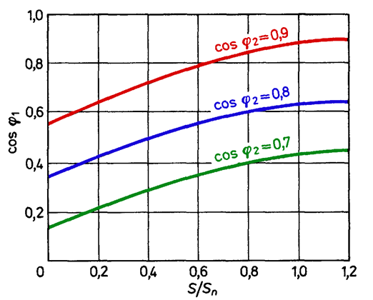
Fig. 6.8. Relation between power factor of primary transformer side and loading, at different power factors of secondary side loading.
Reactive power compensation in industrial receiving devices
Batteries of parallel capacitors are the commonly used for power factor improvement in industrial enterprises. Capacitor connected to the network uses capacitive reactive power, which is equivalent to supplying inductive reactive power to the network.
Four types of compensation with the use of parallel capacitors are distinguished: individual, group, central and mixed.
Individual compensation – capacitor battery is directly connected to the receiver terminals.
Advantages of such compensation are: size reduction of all the network elements, lack of separate devices protecting the battery and switchgear and lack of discharging resistors. Disadvantages of such compensation are: generally higher number and power of capacitors is used than in other types of compensation and after switching-off the receiver the capacitor is not used.
Individual compensation shall be applied where the power of the receivers is large enough, where there is a long enough operating time and the distance from the supply system is sufficient, or where they are the only reactive power receivers among receivers of real power.
Group compensation – capacitor batteries connected to local substation bus-bars (reactive power compensation of receivers fed from this substation).
Central compensation – capacitor battery in main supplying substation on the side of high (medium) or low voltage.
Mixed compensation is the application of two or three before mentioned types of compensation
The type of compensation is determined by the economic calculation.
Reactive power compensation in industrial …
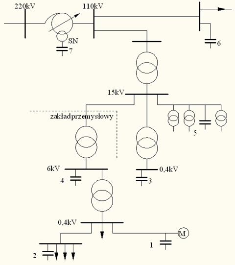
Battery 7 is an example of central compensation in HV network; it is connected to the third winding of a 220/110 kV autotransformer and battery 6, connected to the bus-bars of a 110 kV substation. Battery 5 is an example of central compensation realized in distribution network; it may be installed on the pole of main MV line, supplying several distribution- transformer MV/LV substations. Batteries 4 and 3 are examples of individual compensation of a transformer on the MV and LV side. Battery 2 realizes compensation of a group of receivers. Capacitor 1 realizes individual compensation of motor M.
REAL POWER AND ACTIVE ENERGY
Active energy is generated in generating units (power plants). Active power flowing through the network changes itself according to the character of customers (single shift or multi shift industrial company – Fig. 6.3, utility customer – Fig. 6.4), hour of the day, season of the year, etc.
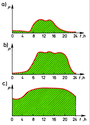
Fig. 6.3. Changeability of real power consumed during 24 hours by industrial companies: a) single-shift company; b) two-shift company; c) three-shift company
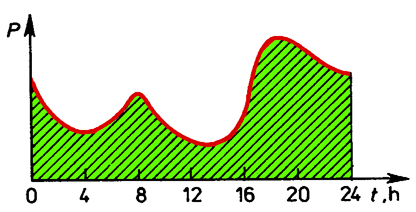
Fig. 6.4. Changeability of real power consumed during 24 hours by public utility loads
15-minute average values of power are usually used to plot the graph of real power fluctuations in time. They are chosen in such a way that the area of the rectangle covers the area under the curve (Fig. 6.5).
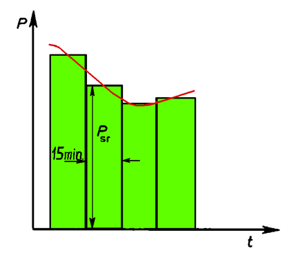
Fig. 6.5. Averaging of a stepped power diagram.
With more than one rectangle, the variation curve changes from a step to a continuous curve in the graph. The area between the 24-hour power curve and the time axis represents, on a certain scale, the energy transmitted through the network and delivered to customers within 24 hours.

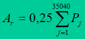
In case of 15-minute time segments
where: Pj – average 15-minute values of power.
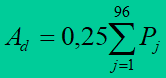
Daily power charts throughout the year are put together in an ordered power chart. In this chart, the average power in 15-minute time segments is set according to their values, i.efrom the highest peek power, which can be met during a year, to the lowest power. The base of the graph is the total number of hours in a year, it is 8760 (Fig. 6.6).
Fig. 6.6. Example of an ordered annual load chart
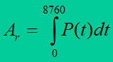
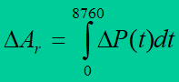
The area between the power curve and the time axis presents quantity of generated energy, sent through the network or consumed by a receiver during a year, so
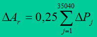
or at 15-minute time segments
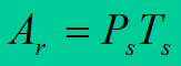
The area Ar is substituted by an equivalent rectangle of height Ps. The base of the rectangle is called annual duration of peek power usage Ts. It is number of hours during which at generation, transmission or consumption of the peek power Ps the same energy Ar is generated, transmitted or consumed as in reality in the whole year
Annual duration of peek power usage characterizes making use of devices. The closer its value to 8760 h, the better making use of the network.
So called annual average load factor also characterizes making use of the network very well
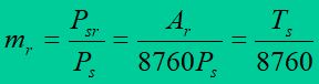
where: Psr – average annual load.
Power and Energy Losses
Real power load losses
These are losses in series resistances R
The following formula may be used for a two-winding transformer
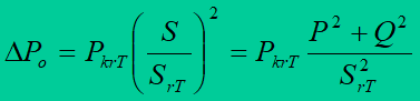
where: PkrT – real power load losses in the transformer at nominal load, SrT – rated power of the transformer.
Overhead lines
Real power no-load losses are calculated with a more accurate analysis of overhead lines with a voltage of 110 kV and higher. These are losses caused by the insulation leakage and the corona phenomenon. Their value is usually determined experimentally. Existing empirical methods do not give too precise results.
Cable lines
No-load losses are calculated more accurately for MV and HV lines. Those loses are caused by the ionisation and the phenomenon of dielectric hysteresis. They are computed from the formula
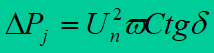
in which: C – working capacitance of a single cable core, tg(δ) – dielectric loss factor of the cable insulation.
Transformers
No-load losses ΔPFe of active power in transformers are estimated at more accurate network computations. They are usually neglected in the transformers of upper voltage lower than 110 kV. These are Joule-Lentz losses on heat, caused by inductive eddy currents in the transformer core and losses caused by the phenomenon of magnetic hysteresis in the core.
Capacitors
The losses are very small and they are about 2 – 5 W/kvar of the power installed in the battery. These losses are caused, similarly like in the cable, by the ionisation and the phenomenon of dielectric hysteresis. They are taken into account only at more precise calculations.
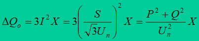
Reactive power load losses
These are reactive power losses in series reactances X of the devices
The following formula may be also used for a two-winding transformer

where: uXr – reactive component of a short-circuit voltage of the transformer, in percents.
Reactive power losses in the series reactor may be also computed from the relation
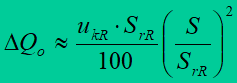
where: ukR – reactor short-circuit voltage in % , SrR – rated power of the reactor.
Reactive power no-load losses
Overhead and cable lines
No-load reactive power losses are calculated with a more accurate analysis of overhead lines with a voltage of 110 kV and above and in MV, HV and EHV cable lines. These losses occur in capacitance between phase conductors and between phase conductors and ground. They are calculated on the basis of the formula
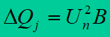
where: B – capacitive susceptance of the line.
Transformers
No-load losses of reactive power in transformers are estimated at more accurate network calculations. Those losses are caused by magnetization of the transformer core, and are calculated from
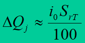
where: i0 – transformer magnetizing current expressed in percents.
Active energy load losses
Power losses in the network change in time, similarly like power flowing through the network. Power losses in the whole year may be also tabulated in the form of ordered graph, i.e. from maximum power loss (corresponding to the flow of the peek power) ΔPmax to minimum loss ΔPmin . The base of the graph is the total number of hours in a year, i.e. 8760 (Fig. 6.9). This diagram is much steeper than corresponding to it ordered graph of power.
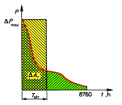
Fig. 6.9. Example of an ordered annual graph of power losses
It’s the result of the proportionality of power losses to the square of power flow. The area between the loss curve and the time axis presents the quantity of energy lost in the network during a year, so
Because average 15-minute time segments are considered, to which average values of losses correspond, then
METHODS OF LOSSES DECREASING
Decreasing of the active power and energy losses in the power networks is the main goal of electric power engineers. The methods of their reduction may be divided into:
⦁ exploitation methods,
⦁ investment methods.
The means of exploitation are non-investment resources and should be used first. Exploitation methods based on loss reduction can only result in a relatively small reduction in losses. Significant effects can only be achieved through investments in the network.
The most important exploitation measures are:
1. Maintaining as high a voltage level as possible in the networks. This reduces longitudinal losses. These losses are inversely proportional to the square of the voltage (they constitute about 80 – 85% of the network losses). With the rise of the voltage shunt losses are also increased, but their share in the total losses is much smaller. Appropriate voltage levels are maintained by controlling the voltage in the network.
2. Reduction of reactive power consumption from the network, which means reduction of actual power losses.
3. Application of efficient network schemes, for example meshed systems instead of open layouts (LV and 110 kV networks).
4. Optimization of network configuration split points by sectioning switches
The most important investment measures are:
1. Introduction of optimal structures of nominal voltages in the network, for example in the Polish conditions 400/110/20/0,4 kV is the optimal structure of the voltages in the networks. The networks of other voltages should be rebuilt to optimal. The networks 0,66 kV, 6 kV and 10 kV in industrial companies are exceptions here. Those voltages serve to feed the asynchronous motors and cannot be eliminated.
2. Elimination of additional transformation steps from the network. Transformation from 20 kV or 15 kV to 10 kV or 6 kV should be avoided in the networks of industrial enterprises. MV networks ought to be supplied from the 110 kV network.
3. Installation of new transformers with lower losses.
4. Construction of new overhead and cable lines. Shortening of the line lengths and the reduction of losses will be gained thanks to that.
5. Replacement of conductor cross-sections in overhead lines with greater ones.
6. Installation of devices for the reactive power compensation and batteries of capacitors, synchronous motors and synchronized asynchronous motors.