6 Electric Power Network
ELECTRIC POWER NETWORKS
An electric power network is a set of cooperating power lines and substations dedicated to the transmission and/or distribution of electricity in a defined area.
The following basic concepts are introduced:
– network structure – unequivocally defined network structure with parameters of individual devices,
– network configuration – unequivocally defined layout of a given network structure obtained by switching on and off, made in a set of its elements; the following configurations are distinguished: normal, emergency and post-emergency,
– network state – a set of values of functions defined at nodes and branches of the network, determining univocally the state of network operation; most often these are voltages in nodes and powers (currents) in branches.
Due to their role in the electricity supply process, power grids are divided into:
– transmission networks of nominal voltages of 220 kV and higher and
– distribution networks of nominal voltages of 110 kV and lower.
Networks of various types have specific layouts of lines and substations resulting precisely from the required reliability of operation and ways of protection of lines, transformers and substations. The names of network systems are related to their normal operation configuration.
Basic network layouts are:
– open network and
– meshed network.
Meshed networks have meshes, open networks shall not have meshes.
ELECTRIC POWER NETWORKS
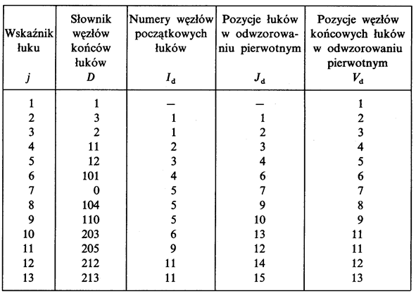
A typical example of an open network is a radial layout.
It is constructed in such a way that electric energy of each load is taken only in one point of network supply and may be led to the load only through one route. This route is formed by a line from the power substation to the receiver connected at the end of the line – see Fig. 5.1.
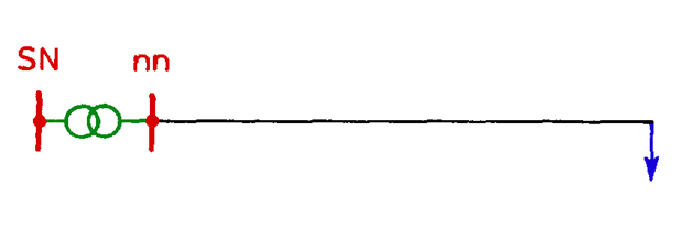
Fig. 5.1. A simple radial system with a single load at the end of the line SN = MV, nn = LV
Radial layouts can be more complex.
Fig. 5.2 presents branched radial system, connecting lines of different voltages with the use of transformers.
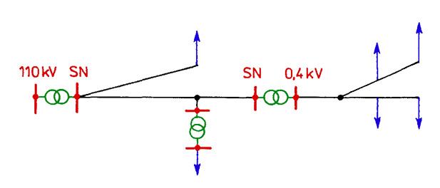
Fig. 5.2. Radial system with series connection of transmission links of different voltages through a transformer substation SN = MV, nn = LV
Arterial layouts are other kinds of open layouts. In this system loads are distributed along a single line, which is called arterial line (Fig. 5.3).
Fig. 5.3. LV arterial layout SN = MV, nn = LV
The lack of reserve is a feature of the open layouts. Fault at any point of the network results in the loss of electricity supply to some, and sometimes even all consumersRestarting the power supply is possible only after the damage has been repaired. With such systems, a selectively operating protection system is necessary.
As a result, open layouts may be applied where there exists high reliability of transmission elements and low reliability requirements of the customers. For example LV lines used in electrical installations show high reliability. In these installations, the gradation of the nominal current values of the fuses used is widely used.
Radial layouts can be successfully used in supply installations for single receivers in industrial enterprises, where the receiver does not need to have an emergency power supply. Radial layouts are commonly used in LV rural networks.
In the case of industrial loads, which require higher reliability of supply, two-radial systems are applied (Fig. 5.4). One of the lines is loaded and the other constitutes back-up.
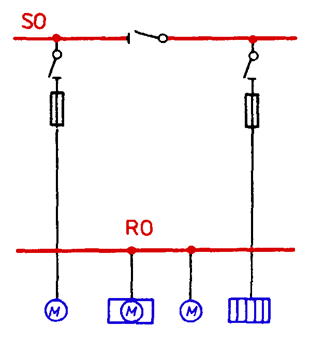
Fig. 5.4. Two-radial layout of an industrial LV network
The feature of meshed networks is the ability to power each client from several independent sources.
These sources may be separate substations or busbar sections in the same station, but each section must be powered by a separate transformer. Therefore, line connections in these networks must be between independent sources. This is due to the need to supply back-up consumers in order to meet the basic requirement for networks – the reliability of the electricity supply.
Networks with meshed structures may work in:
– meshed,
– partly open,
– open configurations.
A network operating in meshed configuration has its switches closed, so energy to each load can flow from all the sources installed in it. The 400 kV and 220 kV transmission networks belong to the networks working in meshed configurations. In many European countries LV urban grids (Fig. 5.5) also operate in meshed configurations. These networks are characterized by very high reliability of customers’ supply.
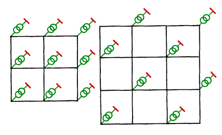
Fig. 5.5. Examples of grid layouts
In a network with partly open configuration electric energy can flow only from one source to some customers. The remaining loads in the network are fed from many sources. An example of such a network is 110 kV network (Fig. 5.6).
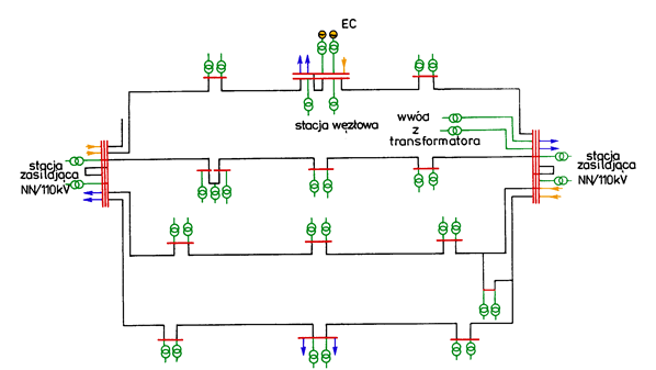
Fig. 5.6. 110 kV network model for a town with population 100 – 200 thousand,
Stacja zasilająca NN/110 kV = feeding substation HV/110 kV
Stacja węzłowa = node substation, wwód z transformatora – input from transformer
Open configuration is obtained from meshed structure by such switching over in the network in such a way that electric energy flows to each load only from one source.
Basic layouts of networks with meshed structures, operating in open configurations, are:
– loop layout,
– two-line closed layout,
– split grid layout.
Loop systems are created in such a way that line links, to which customers are connected, are fed from two sources. They are applied both in LV networks and MV networks (Fig. 5.7).
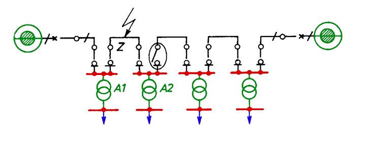
Fig. 5.7. Example of a loop of a MV line, Z = short-circuit
Each line link between two sources is split. Two half-loops re created which are powered from different sources. Customers are supplied with power in such a way that power can be switched on from another source in post failure configurations.
The two-line systems are used in MV networks to feed loads requiring particularly high reliability. They work as split by introduction of divisions (Fig.5.8). Possibility exists to make splitting and switchover at load points.
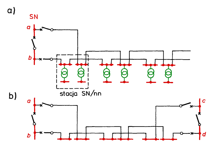
Fig. 5.8. Two-line system: a) lines fed from the same substation, b) lines supplied from different substations
Split grid system is applied in Poland in LV networks in districts with traditional buildings (Fig. 5.5). The splitting is made at service points (connectors). It is expected that this layout will work in meshed configuration in the future.
Meshed networks, working in split configurations, are characterized by relatively high reliability, but far lower than networks operating in meshed configurations.
STRUCTURES OF EL. POWER SUBSTATIONS
An electric power substation is an integral part of a network, and its layout results from the existing network structure.
MV/LV transformer distribution substations are load points in the MV network and, at the same time, they are supply points of the LV network.
Fig. 5.9 presents typical structure of a single-transformer substation, used in urban networks, equipped with two switchgears: medium and low voltage. Up to three MV lines can be connected to this substation.
They use transformers with the following nominal powers: 250 kVA, 400 kVA and 630 kVA. A fuse is used to protect against faults. An overload switch is used for switching on and off operating currents. The supply bays in the LV switchgear are equipped with load-breaking disconnectors with integrated fuses, which protect supplying LV lines against short-circuits and overloads.
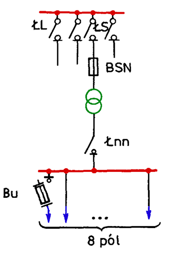
Fig. 5.9. Typical MV/LV single-transformer substation of an urban network
Fig.5.10 presents a structure of a MV/LV two-transformer substation, fed from a two-line system. This structure is characterized by high level of reliability. It is applied for feeding important urban and industrial customers.
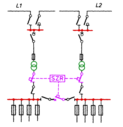
Fig. 5.10. MV/LV two-transformer substation equipped with automatic stand-by switching-on system
The substation is equipped with load-breaking disconnectors in MV feeder bays, which enable switching over in line links supplying it. Arrangement: load-breaking disconnector – fuse is used in the MV transformer bays in the case when the substation is equipped with MV/LV transformers of power up to 800 kVA. Circuit-breakers are applied at higher powers. The substation has two sections of LV switchyard and is equipped with automatic stand-by switching-on system. In the case when the voltage collapse exists on one of the transformers, automatic stand-by switching-on system switches over the LV switchyard section without voltage on supply from the second transformer. Both sections of the LV switchgear are then supplied from one transformer.
110kV/MV substations are most frequently two-transformer substations with powers equal to: 6.3, 8, 10, 12.5, 16, 20, 25, 31.5, 40, 50, 63 MVA. The layout of the MV switchgear depends on the power of the 110kV/MV transformers
installed in it. The simplest layout is a switchgear with single bus-bar divided into sections with a circuit-breaker (Fig. 5.11).
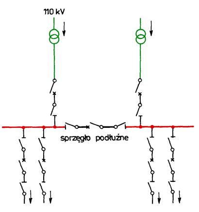
Fig. 5.11. Simple layout of a MV switchgear with single bus-bar system with two sections
The dividing into sections of the bus-bar systems is indispensable to ensure supply continuity. In the event of a failure of the 110 kV power line or the 110 kV/MV transformer, the system allows switching operations to be carried out that provide partial or total coverage of the customer’s demand.
Double bus-bar system is used for 110 kV/MV transformers with higher power. One of the systems is divided into sections with the help of bus switches (a circuit-breaker and disconnectors) – Fig. 5.12. Such a connection is called bus-bar coupling.
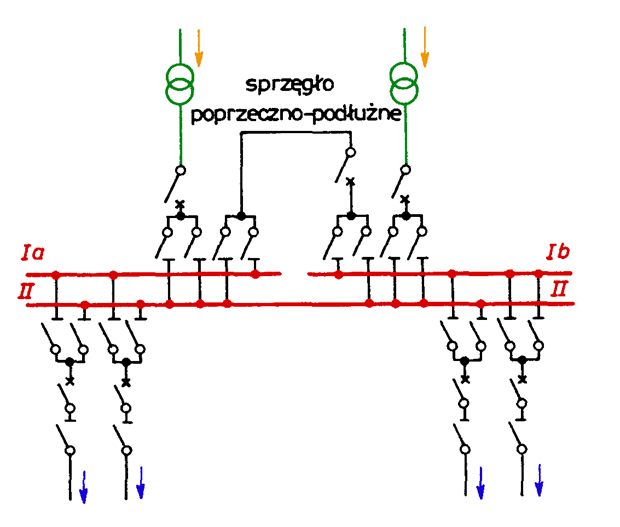
Fig. 5.12. MV switchgear layout with double bus-bar system (I, II); system I divided into two sections
110 kV mesh-type substations of the H-type, and most frequently of the H3-type are mainly applied in 110 kV line links (Fig. 5.13) The system H3 is equipped with three circuit-
breakers: in feeder bays and in the cross-bar. In short 110 kV lines the circuit-breakers may be located in transformer bays.
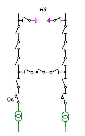
Fig. 5.13. 110 kV mesh-type substation – system H3 (Os – fast disconnector)
In nodal 110 kV/MV distribution transformer substations (third transformer is installed or more than two 110 kV lines are brought to the substation) single systems of bus-bars are used, divided into two sections with sectional bar circuit-breaker of the structure similar to the MV switchgear, presented in Fig. 5.11.
In 110 kV network nodes, in 400 kV/110 kV or 220 kV/110 kV substations, double and sometimes even triple bus-bar systems are used in a 110 kV switchgear. Fig. 5.14 presents an example of a nodal 110 kV switchgear equipped with two systems of bus-bars with crosswise bus-coupler circuit-breaker. The switchgear is fed from EHV/ 110 kV substation. Distribution of electric power into 110 kV line links takes place in it. It may also feed 110 kV/MV transformers.
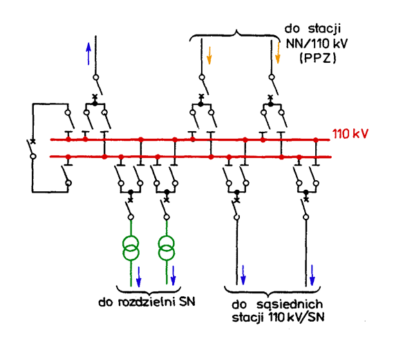
Fig. 5.14. 110 kV switchgear with double bus-bar system, applied in the nodes of the network
In nodal substations of 400 kV voltage solution with double, sectionalized bus-bar system with two circuit-breakers in each bay is assumed (Fig. 5.15). The system has very high reliability. Transformers with power 125, 160, 250, 330, 400, 500 MVA are applied in EHV substations.
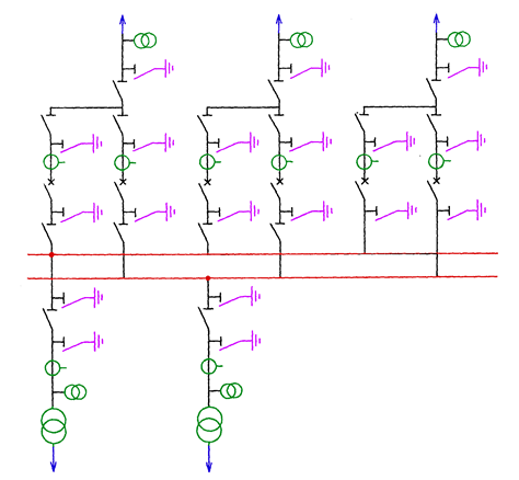
Fig. 5.15. Connection diagram of a large 400 kV substation
EQUIVALENT SCHEMES OF NETWORK ELEMENTS
The following elements of electric power networks are the most commonly used in calculations:
– electric power lines,
– transformers,
– reactors,
– capacitors.
For the network calculations those devices are represented, according to the kind of calculations and their nominal voltages, either as four-terminal networks or as two-terminal networks.
Impedances and admittances of a line are evenly distributed along the line, but this should be taken into account only in case of long EHV lines (220 kV, 400 kV and 750 kV). In most cases we use equivalent scheme in the shape of four-terminal -type network (Fig. 5.16), or even in simplified calculations of LV, MV and HV lines we use the scheme in the shape of two-terminal network (Fig. 5.17).
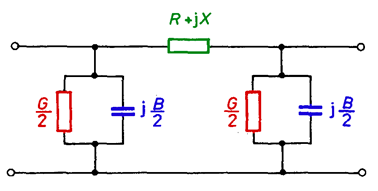
Fig. 5.16. Equivalent scheme of a line in the shape of -type four-terminal network
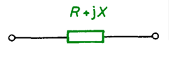 Fig. 5.17. Equivalent scheme of a line in the shape of two-terminal network R, X
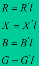
Per-unit impedances and admittances R’, X’, B’, G’ related to 1 km of line length are characteristic parameters of the line. Total impedances and admittances are received multiplying them by lengths:
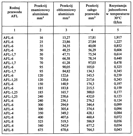
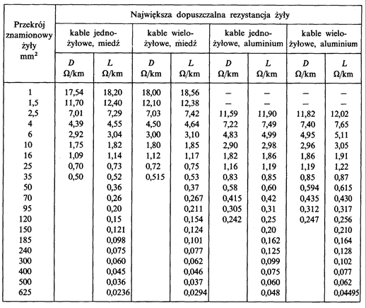
In the case of the lack of the tables it may be computed from a formula
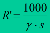
where: – specific conductivity of conductor material,![]()
s – cross-section of a conductor [mm2].
In practice, to find per-unit reactance X’ we use suitable charts and tables. Per-unit reactance of overhead line conductors depends on the distances between the conductors, arrangement of the conductors on poles, their diameter,
conductor construction, and magnetic features of materials of which the conductors are made.
![]()
where: bL1,L2, bL1,L3, bL2,L3 are the distances between appropriate conductors
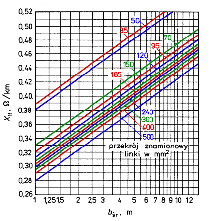 Fig. 5.18. Per-unit inductive reactance of steel-aluminium conductors of three-phase single-circuit lines in relation with the distance between the conductors at different nominal cross-sections
Per-unit inductive reactance X’ of cable lines depends on distances between the cores, cores diameter and shape, cable construction and eventual influence of magnetic materials in the cable. Graphs of variableness of per-unit reactance of cables with core insulation have been presented in Fig. 5.19 and with screened conductors in Fig. 5.20 as a function of nominal voltage and core cross-section.
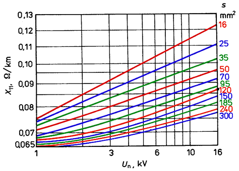
Fig. 5.19. Per-unit inductive reactance of cables with core insulation
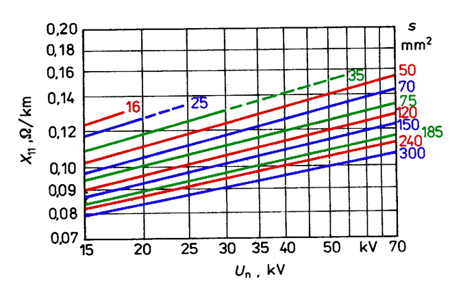
Fig. 5.20. Per-unit inductive reactance of cables with screened conductors
Per-unit conductance G’ of a line in overhead lines, caused by corona losses, is usually neglected. In cable lines there are losses caused by ionisation and dielectric hysteresis. The ionisation originates in the cable because of existence of air bubbles in the insulation. Losses caused by the dielectric hysteresis arise as the result of the electric field intensity changes. For a three-phase cable they are calculated using the following formula
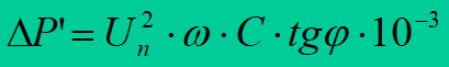
where: C – working capacitance of line conductors, tg – coefficient of dielectric lossiness.
The conductance calculated using the following formula
Per-unit capacitive susceptance B’ of a line
Conductors, together with existing between them layers of insulation, may be treated as a system of capacitors.
Two capacity types are distinguished:
– working capacitance Cr of one cable conductor, indispensable for calculation of the line charging current,
– capacitance for zero-sequence component C(0) of one cable conductor, necessary to calculate earth-fault currents.
Cables with radial field
An insulation of a cable conductor with radial field may be treated as cylindrical capacitor (Fig. 5.21). The values of the capacitance of those cables are given in table 5.3. The capacitance: working and for zero-sequence component for cables with radial field is the same.
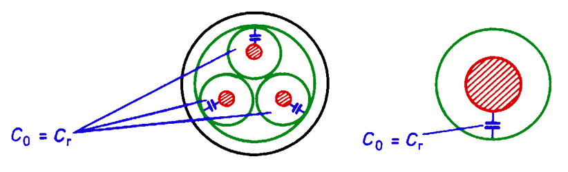
Fig. 5.21. Shunt capacitance of cables with radial field: three-core and single-core
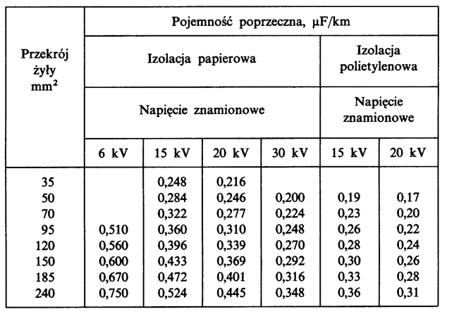
Table 5.3. Per-unit shunt capacitance of cables with radial insulation
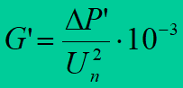
Cables with core insulation
Working capacitance of a cable with core insulation is the total capacitance of one core, consisting of (Fig. 5.22):
– partial capacitances between conductors and metal sheath – C(0)
– partial capacitance between conductors – C1
In a symmetrical three-phase arrangement the working capacitance is
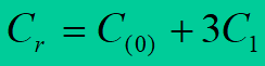
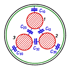
Fig. 5.21. Shunt capacitance of cables with radial field: three-core and single-core
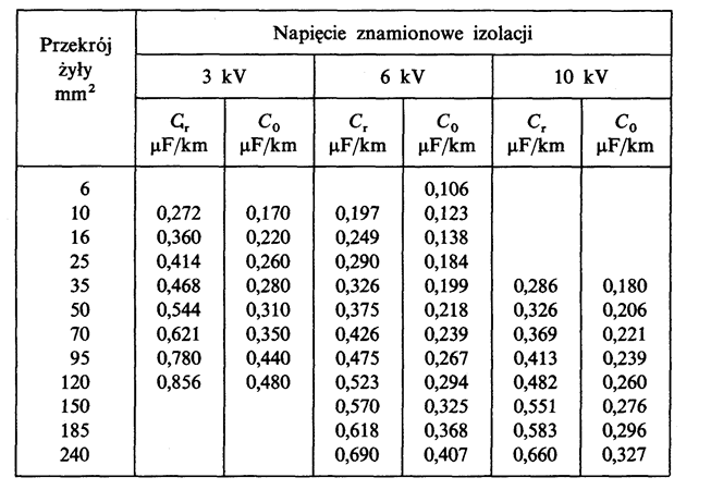
Table 5.4. Per-unit capacitances for zero-sequence component and working capacitances of cables with core insulation
Overhead lines
In overhead lines the relationship between capacitances is the same like for cables with core insulation (5.6) – Fig. 5.23.
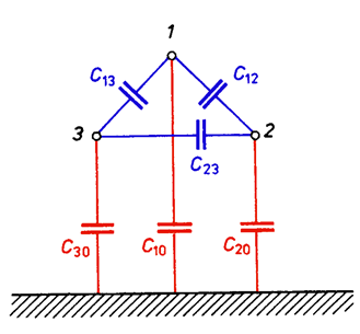
Fig. 5.23. Arrangement of partial capacitances of a single-circuit overhead line
Transformers
The two-winding transformers with upper voltage 110 kV and higher, at precise calculations, are represented either by
T-type or type four-terminal networks (Fig. 5.24).
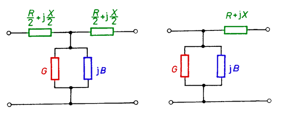
Fig. 5.24. Equivalent schemes of a two-winding transformer in the shape of four- terminal networks: a) T-type, b) -type
The two-winding transformer, at less precise computations, and transformers with upper voltage lower than 110 kV are represented as two-terminal networks R, X.
Basic parameters for the transformers are:
• rated upper UrH and lower UrL voltages,
• nominal ratio tr,
• nominal currents: upper IrH and lower IrL,
• rated power SrT,
• short circuit voltage ukr,
• active power losses in windings PkrT,
• power losses in transformer core Pfe,
• no-load current i0.
In network calculations we use total resistance RT and total reactance XT of the transformer. Their value depends on the assumed reference voltage (voltage of upper or lower winding). The following relation is valid:
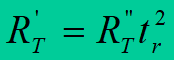
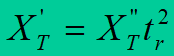
where: R’T and R”T – transformer resistances related to upper and lower voltage respectively, and X’T and X”T – transformer reactances related to upper and lower voltage, respectively.
Resistance RT is determined from the formula
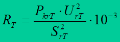
where is expressed PkrT in [kW], UrT in [kV], SrT in [MVA].
Reactance XT is determined from the formula
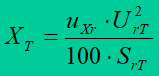
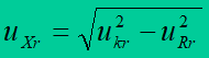
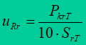
where is expressed uXr – reactive component of a transformer short-circuit voltage in percents, uRr – active component of a transformer short-circuit voltage in percents; UrT is given in kV, SrT in MVA.
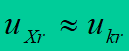
In transformers with short-circuit voltage greater than 10% the following assumption is made:
Conductance representing real power losses in the core of the transformer is computed from the formula
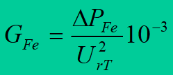
where is expressed ΔPFe in kW, UrT in kV.
Susceptance is calculated from the approximated formula
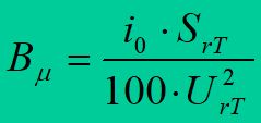
where is expressed i0 in percents, SrT in MVA, UrT in kV.
Current limiting reactors
Current limiting reactors are produced for short-circuit voltages 3% – 15% and nominal currents up to 2000 A. They are applied in networks of voltages 6 – 20 kV and sometimes 30 kV.
Reactor’s resistance constitutes only about 1% of its inductive reactance and may be neglected in the calculations. Because of that the reactor is represented as a two-terminal network with reactance XR (Fig. 5.25).
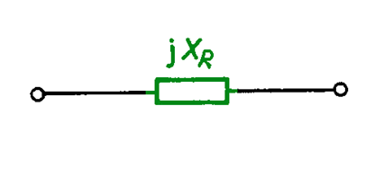 Fig. 5.25. Equivalent scheme of a current limiting reactor
Basic parameters for a reactor are: rated voltage UrR, nominal current IrR and short-circuit voltage ukR.
Reactor’s reactance XR can be calculated from the formula
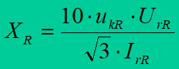
where is expressed ukR in percents, UrR in kV, IrR in A.
Capacitors
Resistance of a capacitor constitutes only 2‰ – 5‰ of its capacitive reactance and practically can be neglected in calculations. Regarding this a capacitor is represented as two-terminal network with reactance XC (Fig. 5.26).
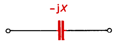 Fig. 5.26. Equivalent scheme of a capacitor
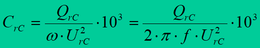
Basic parameters for a capacitor are: nominal voltage UrC and nominal power QrC. Nominal capacitance CrC in F is often given. It may be computed, having rated power in kvar and voltage in kV, from the formula
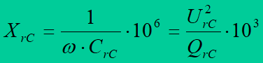
Reactance is calculated from the formula
DIGITAL MODELING OF A NETWORK
The two basic concepts are introduced:
a node (bus) of a network – any point in the network with given denotation; the most frequently they are: sections of bus-bars in substations, feed points of the network, terminals of transformers, receivers and switches and points of branching,
an arc of a network – a network element connecting two neighbouring nodes with specified direction; the most frequently they are: line segments, switches, two-winding transformers, reactors, capacitors, or the sets of these elements connected in series (for example switch – line – switch).
All the nodes in the network should be denoted. Primary denotations are used in the process of preparing data for network calculations on a computer. In general, there is only one rule: the same denotation must not be used for more than one node. Either existing denotation of nodes in the network is used or the principle of uniform denotation of objects and devices, which shall be applied in power engineering. Alphanumeric denotation is often used in networks of voltages 110 kV and higher, where the components are the first letters of the substation name, for instance: JAN 211, GDA 112. Digits mean voltage code and a number of a section in the substation and a number of a regional dispatching center area.
Secondary denotation is applied during computer calculations. Nodes and arcs are numbered with consecutive natural numbers.
Digital network model is the base for calculations on computers. For technical and economical calculations it should contain representation of the network configuration (topology) and its technical and economical parameters. There are two kinds of the network representation:
– primary representation, based on primary denotations of the nodes, used in the process of data preparation and calculation results output,
– secondary representation, based on secondary denotations of nodes and arcs, usually numbered automatically taking into account optimisation of calculation algorithms. Its form depends on the network layout and on the kind of calculation algorithm.
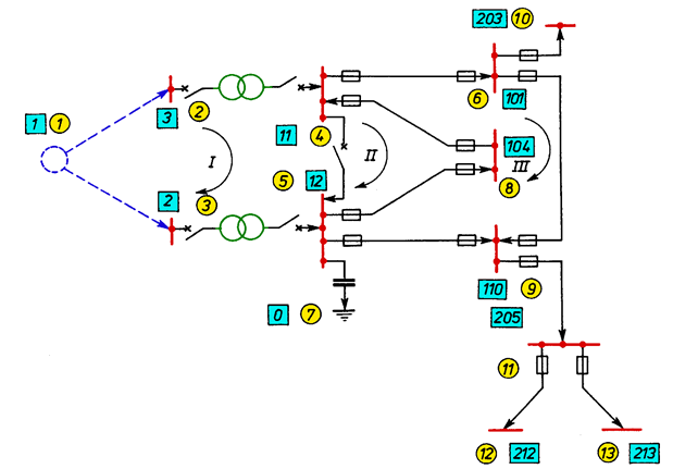
Fig. 5.27. An example of electric power network (numbers in rectangles represent primary denotation of nodes, and numbers in circles – their secondary denotation)
Primary representation formed in the process of data preparation contains the following sets:
– a set of catalogues,
– a set of data and auxiliary coefficients,
– a network structure representation,
– a network configuration representation.
The set of catalogues should contain catalogues of all kinds of network devices, which take part in the calculations. E.g.:
– catalogues of overhead and cable lines,
– catalogues of transformers,
– catalogues of switches,
– catalogues of reactors and capacitors.
Correctly prepared catalogue should contain two parts. The first part should contain: catalogue name, date of its forming or of the latest updating and present number of items in the catalogue. Parameters of devices represented in the catalogue are placed in the second part. A separate row (record) should be reserved for each type of a device. Definition of device identification number, element type, nominal voltage and other information required for calculations is necessary.
An example of a catalogue of cable lines is presented in table 5.5.
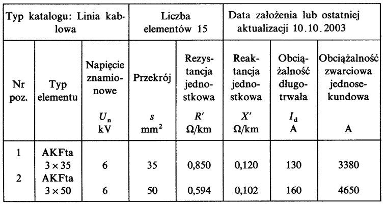
Table 5.5. Catalogue of cable lines.
The first part of the representation of the network structure contains information such as the name of the network structure, the date of creation of the sets or their last update and the number of arcs m and nodes n. The second part contains a full list of arcs (Table 5.6) and nodes (Table 5.7).
The list of arcs includes the following items:
• denotations of nodes connected by the arc,
• the name of the catalogue of devices represented by the arc; in case when the arc represents more than one device, the names of the catalogues are given and positions in those catalogues for the rest of the devices. If a main device is in the whole representation accompanied by only one device type, for example switches, than the names of the catalogue of auxiliary devices in the arcs may not be given,
• the numbers of positions in the catalogue of devices,
• the lengths of arcs representing lines; 0 or 1, according to the needs, is assumed for the rest of devices,
• supplementary information, like for example arc code, date of a device construction, date of modernization, device cost is located in the table of arcs.
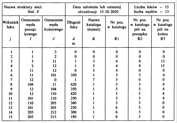
Table 5.6. Information defining a network and complete list of arcs in primary representation of a network from Fig. 5.27
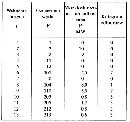
Table 5.7. Complete list of nodes in network primary representation
The following items are given in the list of nodes:
• denotations of nodes,
• powers (currents) drawn from or fed to the node,
• supplementary information, for example capability of nodes – feed points, categories of customers in nodes – load points.
Data for arches and nodes may be supplemented during the operation of the database with data from telecontrol or from computer links, such as:
• measurements of powers and currents in arcs,
• measurement of voltages in nodes.
Network configuration representation
A number of configurations, differing in the circuit arrangement, are usually analysed for each network structure in the calculation of electricity networks. For each of the analyzed configurations, the set of arcs and nodes in the configuration should be given. Back-up devices, repaired devices and tripped after fault are understood as out of action elements.
Only denotations of nodes: initial and final are given for every out of action arc (table 5.8). Only the number of the node is given for every out of action node. The rest of information about out of action arcs and nodes is contained in the complete network representation. The set of out of action elements is preceded by information containing: the name of network structure, the name of configuration, the date of the set creation and the number of out of action arcs and nodes in the set.
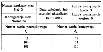
Table 5.8. Information defining network configuration and a list of out of action arcs in the network from Fig. 5.27.
Secondary representation example for distribution network working in radial configuration.
A computer converts network primary representation into secondary representation – individually for each of analysed network configurations. Lists of arcs and nodes are converted, but the sets of supplementary data and the sets of catalogues remain unchanged.
At the beginning the computer introduces secondary numeration of nodes. At the same time it forms a dictionary of the nodes (tab. 5.9) enabling transition from secondary numeration to primary numeration (vector D [1:n]).
So called inversion structure is introduced to represent network topology. Vector Id [2:n] is formed, in which for every arc [i, j] element with index j, 2 ≤ j ≤ n is appointed. The index is equal to the number of the node at the end of the arc of value Id[j] = i equal to the number of the node at the beginning of the arc. Because of the following feature of the radial network – in each node finishes only one arc, the vector Id at the same time represents the topology of network configuration.
The following vectors are built to form the secondary representation (tab.5.9):
– Id [2:n], in which position index j, 2 ≤ j ≤ n, is equal to the number of the node of the arc end [i, j] in the secondary representation, and element Id[j] is equal to the index of this k, 2 ≤ k≤ m in the primary representation in the full list of the arcs (table 5.6),
– vector Vd [1:n], in which position index j, 1 ≤ j ≤ n, is equal to the number of the node of the arc end in secondary representation, and element Vd[j] is equal to the index of this node k, 1 ≤ k ≤ n, in the primary representation in the complete list of nodes (vector V).
ELECTRIC POWER NETWORKS
Information contained in the vectors Jd and Vd enable to choose, in a simple way, the following data from the primary representation: node number in the primary representation, catalogue name, position in the catalogue, arc length, node load, etc.