13 Operation of a synchronous generator in an electric power system and problems of stability (fin)

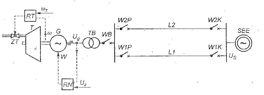
The goal of this task is to investigate stability problems of synchronous generator. The used physical model of the generation unit during the laboratory training is presented in figure 1. The basic phenomena which are going to be investigated during the training are local and global stability

Local stability – small disturbace stability

The generation unit is connected to EPS, which is the complex system consisting of many lines, loads and other generation units. Accoring to Thevenin’s Law we are able to transform this system into one impedance and voltage source, called infinite bus (bus 3 in fig. 2).  Since R<<X resistance can be neglected.

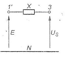
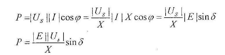
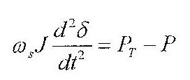
Using the presented simplification is it possible to formulate the equation which couples P and δ variables with each other. The final equation is presented in (1).

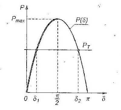
According equation (1) we may create a P(δ) characteristic, which is presented in figure 3

Because the E is coupled with synchronous machine rotor, we may interpret that changes of δ relate to the angle physical position of the turbine, axis and rotor. This is why the angle δ is called angle of rotor position. The change of this angle in time is determined by the second law of dynamics for the rotation motion equation 2.

Jε = ΔM  (2)

where J is the moment of inertia of unit rotor mass,

ΔM is difference of driving and braking torques,

ε is acceration caused by the difference of torques.

Assuming that the rotor speed is close to synchronous speed equation 2 may presented in following form:

In steady state P_T is equal to P, so acceration ε is zero. Such state is called the state of equilibrium. As you may see in figure 3 synchronous generator working with turbine has two equilibriums.

However not every state of equilibrium may be the stable point of operation.

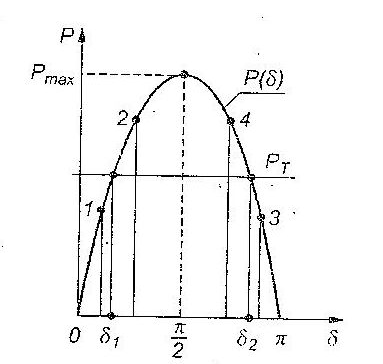
Deviation to point “1” causes arising of positive difference ΔP = (P_T – P), thus according to the equation (3) positive acceleration. The movement is done to the side of increasing values of δ and it is followed by the return to the equilibrium point δ₁ . Deviation to point “2” causes arising of negative difference ΔP , or the negative acceleration. The movement leads to the decreasing values of δ which is followed by the return to the equilibrium state δ₁ . It means that δ, is the state of permanent equilibrium (locally stable).

It is completely different in the state of δ₂ equilibrium. Deviation to the point “3”, causes arising of a positive acceleration e and movement to the side of growing δ values, which means moving away from the point of equilibrium. It is similar at the deviation to the point “4”. It means that δ₂ is the state of unstable equilibrium (locally unstable).

So from the point of view of local stability the considered synchronous generator may operate at P_T < P_max and δ  < π/2

Global Stability – large disturbance stability

Beside various small disturbances there may be present also large disturbances. The examples of such perturbations:

• switching-off strongly loaded line leading out the power to EPS,
• short-circuit on one of the lines and its switching-off after the time t_z ,
• power plants tripping off.

After disturbances of this type there may be present, but not necessary, the loss of system stability consisting in transition to asynchronous work of a synchronous generator or generators being close to the mechanical failure.

To understand the global stability best, two following examples are necessacy to study. Three phase short-circuit occurs close to the terminals of the synchronous generator. In first case short-circuit last t_z1 and in second case short-circuit last t_z2.

For simplicity of considerations it is assumed that the voltage regulator is switched-off. Long time constants of turbine regulation system RT additionally enable to assume in the considerations that the mechanical power in interesting us period of time is constant (P_T is constants).

As it was said in previous part the synchronous machine works in point “1”. When short-circuit appears point of operation changes its position to “2”. During the three phase fault the voltage at the generators terminal is zero so the electrical power is zero as well.  This is a vertical line (because the rotor angle cannot change its value immediately).

During the fault angle changes its value from “a” to “b” (and from point “2” to “3”) – the rotor is accerating. If the fault was not cleared  the angle value would have unstoppably increased (the dotted line). When the fault is cleared in time t_z1 point of operation changes from point “3” to point “5”. Then the electrical power sent to the EPS is greater then mechanical power of the turbine (P_T), so the rotor is decelerating. The energy gained by the rotating masses during the fault are linear to area 1, 2 ,3 ,4 called area of acceleration. Now the rotor has to lose this energy in an area called area of deceleration – area 4, 5, 6, 7. Area 1, 2 ,3 ,4 = area 4, 5, 6, 7.

The angel changes its value from “b” to “c” which is the maximum and then it moves back to angle “a”.

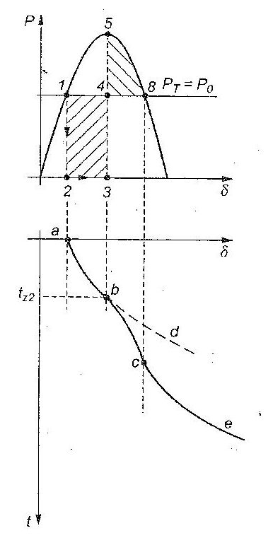
The second case is similar to the first. The difference is longer time duration of fault. Then the acceleration area is bigger and possible decelation area is smaller. As it is presented the in the figure when the generator reaches point “8” the rotor is starting to accelerate and it is losing its stability. Area 1, 2, 3, 4 > area 4, 5, 8.